Received: December 20, 2023; Accepted: May 9, 2024; Published: June 13, 2025
Farm characteristics and exogenous factors influencing the choice to buy land in Italy
1 Department of Agricultural and Food Sciences, Alma Mater Studiorum, Università di Bologna, Viale Fanin 50, Bologna, 40127, Italy
2 Department of Statistical Sciences “P. Fortunati”, Alma Mater Studiorum, University of Bologna, Via Delle Belle Arti, 41, BO, Bologna, 40126, Italy
3 CREA – Research Centre for Agricultural Policies and Bioeconomy, Legnaro (PD), Italy
*Corresponding author. E-mail: silvia.russo7@studio.unibo.it
Abstract. Access to land is one of the key factors of farm growth. However, related research is characterised by important gaps, in particular, facing the change over time in the nature and role of drivers of the land market. The objective of this paper is to identify the endogenous and exogenous factors that affect the decision to purchase land in Italy between 2013 and 2020. Five probit regression models were implemented to understand the role of a set of different determinants in land investment decision. The results show that factors related to capital in machinery and plant, energy production and the presence of a successor or young farmer are endogenous factors that positively influence the purchase decision. The ratio of rented land to utilised agricultural area and of family work units to total work units are endogenous factors that negatively affect the purchase decision. Exogenous factors related to the cost of capital and inflation rate affect the purchase of land in an opposite way, negatively and positively respectively. The role of Utilised Agricultural Area and Value Added per hectare varies depending on the specialisation considered. The research can support policymakers in designing policies to promote the survival and growth of farms, as well as to facilitate land investment by reducing barriers to land acquisition.
Keywords: agricultural land market, land purchase, probit regression model, investment decision, purchase decision.
JEL Codes: Q15, Q12.
Index
3.1. Data and descriptive analysis
3.2.1. Description of the explanatory variables and expected relation
3.2.3. Descriptive analysis of explanatory variables
4.1. Correlation analysis and VIF analysis
Appendix 1. Descriptive analysis of sample farm size based on farm specialization
Appendix 2 Analysis of relationships among independent variables
Land represents a durable, fixed, heterogeneous, and non-reproducible resource and is one of the key productive factors of a farm. The purchase of land is one of the ways through which a farmer can access this fixed productive factor and represents a form of investment in a capital good. Compared to other forms of farm size growth, on the one hand, the purchase of land may require a major financial commitment and thus limits the investment in other productive assets (Jeong et al., 2022; Swinnen et al., 2016). On the other hand, the full transfer of rights allows the new owner to use the land as a collateral asset in order to have greater access to credit (Binswanger et al., 1995; Bradfield et al., 2023; Swinnen et al., 2016). In comparison to investments in other types of on-farm assets, the purchase of land rarely takes place at the same time as it is planned because it is not certain that the farmer will find the supply on the local market meeting his/her needs/capacity (Elhorst, 1993). For the farmer, the availability of land can be one of the main obstacles to the development and growth of the farm (Yanore et al., 2024). The land market is characterised by rigid supply and the purchase of land far from the farm centre would lead to increased costs and downtime (Cotteleer et al., 2008; Schimmenti et al., 2013). For all these reasons, the land market is generally defined as thin and local.
The lack of data availability and the absence of well-structured databases on land transactions, especially in Europe, has influenced and limited the research on the land market (De Noni et al., 2019). Over the years, research mainly focused on identifying the determinants of land value in specific local agricultural land markets or on how agricultural policy payments could influence land value (Baldoni et al., 2023; Czyzewski et al., 2017; Latruffe and Le Mouël, 2009; Michalek et al., 2014; Varacca et al., 2022). However, when analysing the literature relating to the investment decision, there appears to be little ex-post empirical research that takes into consideration the investment in land.
The objective of this paper is to identify determinants that have influenced the farmer’s decision to purchase land in Italy between 2013 and 2020. The work is carried out using FADN data and factors are selected based on a literature review and data availability. The main novelty of the paper is that we use an original analytical framework and a conceptual model developed on the basis of the literature analysis using multiple streams of research, namely structural change in agriculture and the growth of farm size, the investment decision and the land market literature.
The paper continues in Section 2 with the design of the framework. In Section 3 we proceed with the descriptive analysis of the available data and the presentation of the methodology. In Section 4, the results of the analysis are presented and will be discussed in Section 5. Section 6 is dedicated to the conclusions drawn from this study.
In order to contextualize this research, a premise is needed. To the best of our knowledge, there are no studies that have identified the factors that may influence the decision of Italian farmers to invest in land. Consequently, this study and its results should be considered a preliminary exploratory attempt to identify and understand the effects of certain factors selected based on the original analytical framework.
Land is a factor of production that is strongly connected to and not divisible from three other farm inputs such as machinery, (family) labour and buildings (Plogmann et al., 2022).
Over the years, mechanisation and technological innovation have played an important role in improving farmers’ labour management and replacing the labour force leaving rural areas for better paid non-agricultural work. The adoption of machinery and technological innovation, especially when it is expensive and complex, have stimulated farmers to allocate their managerial skills, capital, and farm assets for the production of a few types of output and, thus, farm specialisation. These three factors have contributed to the development of both economies of scale and size. Although technological innovation is accessible to small and large farms, the latter seem to have more financial and managerial capacities, both internal and external, to invest in this factor. Thus, the growth in farm size induced by technological innovation seems to be stronger in large farms than in small ones. According to the theoretical literature, these dynamics generate pressures on small farms that might decide to exit the agricultural sector (Plogmann et al., 2022). In this regard, researchers have identified “off-farm income” as a factor that could play a dual role in the survival of small farms. On the one hand, the income generated by off-farm activities could represent the first step of the farm’s exit from the sector. On the other hand, this source of income could allow the farmer to remain within the agricultural sector because it could contribute to the stabilisation of the farmer’s income and facilitate access to credit, investment in farm assets, and stimulate the growth of farms managed by young farmers (Goddard et al., 1993; Hallam, 1991; Harrington and Reinsel, 1995; Key, 2020; Neuenfeldt et al., 2019; Weiss, 1999; Zimmermann et al., 2009).
Human capital is one of the main factors that can influence a farmer’s investment decision. When talking about human capital, reference is made to demographic characteristics of the farmer and their family. In particular, the age of the farmer and the presence of a potential successor, and the level of education are among the main characteristics that can affect farm size and investment in land. As the age of the farmer increases, the farm enters the so-called maturity and/or decline phase and the farmer may be more reluctant to increase the farm size (Bremmer and Oude Lansink, 2002). The presence of a potential successor could prevent the farm from entering the decline phase and thus positively affect the investment in a fixed input (Huber et al., 2015). Furthermore, the purchase of land could entail a major financial commitment and the application for a bank loan. In this regard, the presence of a young farmer or a successor could positively influence the time horizon of the investment and favour the purchase decision (Elhorst, 1993; Huber et al., 2015; Oskam et al., 2009; Oude Lansink et al., 2001). In addition to these factors, human capital also includes managerial skills that if not possessed by the farmer can be found in the external environment e.g. by turning to advisory and consultancy services (Boehlje, 1992). According to the literature, larger farms may have greater economic and financial capacities to access such services.
The decision to invest in land is not only influenced by structural and socio-demographic characteristics of the farm, but also by exogenous factors such as the macroeconomic environment, land market regulations, and agricultural policies.
The purchase of land represents an investment in a capital good that may require a major financial commitment. In this sense, the cost of capital and the financial position of the farmer could influence the decision and the level of investment. As the interest rate increases, the probability that the farmer is willing to invest and the level of investment decreases.
Land is not only an important production asset of a farm but also a “safe- heaven” asset (Schimmenti et al., 2013), attracting the interest of non-farmers who decide to invest in it to protect the capital value from inflation. An increase in the inflation rate leads to an increase in the price of land and vice versa (Elhorst, 1993; Lawley, 2021; Szymańska et al., 2021; Thijssen, 1996). Policymakers can use land regulation as an instrument to defend the farmers’ position and mitigate potential speculative force in farmland market. Each European Member State has full decision-making power over its own land regulation. In general, Western European countries have a more liberal land regulation than Eastern European countries. Among the Western countries, Italy is one of the European countries with the most liberal land regulation (Swinnen et al., 2016). With the aim of facilitating access to land for medium-sized farms with financial means, many European countries have provided for the right of pre-emption to be exercised either by local governments, as in France, Germany and the Netherlands, or by farmers, as in Italy (Galletto, 2018). In particular, the Italian government introduced this instrument to reduce the fragmentation of Italian farms, to improve the consolidation of the Italian agricultural sector and to facilitate the development of family farms. In Italy, Art. 8 Law n. 590/1965 and art. 7 Law n. 817/1971 establish that the Italian farmer may exercise the right of pre-emption of land if at least one of three cases occurs: a) he/she is the co-owner of the farm, b) he/she is a professional farmer who directly borders land for sale, c) if he/she has been renting the land for at least two years (Legge 590/1965; Legge 817/1971).The right of pre-emption has also been extended to agricultural partnerships (as a rule, simple partnerships, and general partnerships) if at least half of the partners are “owner-operator farmer”. Subsequently, between 2009 and 2016, the Italian State implemented tax concessions to improve the farmer’s position. The law states that: a) the Italian farmer with a family farm does not have to pay income tax or land use tax; b) the Italian farmer is exempt from paying income tax on the use of the land; c) in case of land purchase, when the buyer is a “owner-operator farmer” or professional agricultural entrepreneur, she/he will pay only 1% of the purchase price as tax, while any other buyer will pay 15%. In 2017, the European Parliament called on all Member States to review their land regulation in order to ensure fair access to land and to prevent it from being concentrated within a few large farms (European Parliament, 2017).
In addition to preserving the farmer’s position, land regulation influences the capitalization of subsidies provided by agricultural policies within the value of land and rental rates. Stringent land regulation on the land market and land rental market would reduce the capitalisation of subsidies within the land price and rent. The literature presents both theoretical and empirical studies on whether and how much of the subsidies provided through policies are capitalised within the land price value. From a theoretical study, in a perfect market, decoupled direct payments, coupled direct payments, rural development programmes and environmental payments could be capitalised within the land price. However, empirical studies suggest that capitalisation in a real land market is lower than theorised and depends on many factors such as subsidy type, land supply elasticity and farm credit constraints. In addition to influencing land value, subsidies can also influence a farmer’s investment decision and level of investment. Subsidies were introduced with the main objective of supporting the farmer’s income and represent a form of income not affected by production risks. Consequently, subsidies could positively influence the investment decision and level especially in the presence of an imperfect market.
The identified factors are not independent but interact and influence each other (Zimmermann et al., 2009).
In the literature, four empirical studies concerning the farm size growth were identified that adopted a regression model with the farm size as the dependent variable (Akimowicz et al., 2013; Bremmer and Oude Lansink, 2002; Brenes-Muñoz et al., 2016; Weiss, 1999). In the literature related to investment decision, two empirical researches were identified that also considered land as a form of investment (Elhorst, 1993; Oskam et al., 2009). In addition, Jeong et al. (2022) identified farm economic characteristics that could affect the decision to buy or lease land in Korea by adopting the machine learning algorithm “random forest”. Finally, Ziemer and White (1981) attempted to better estimate farmland demand in Georgia between 1970 and 1978 by accounting for the process underlying the decision to purchase.
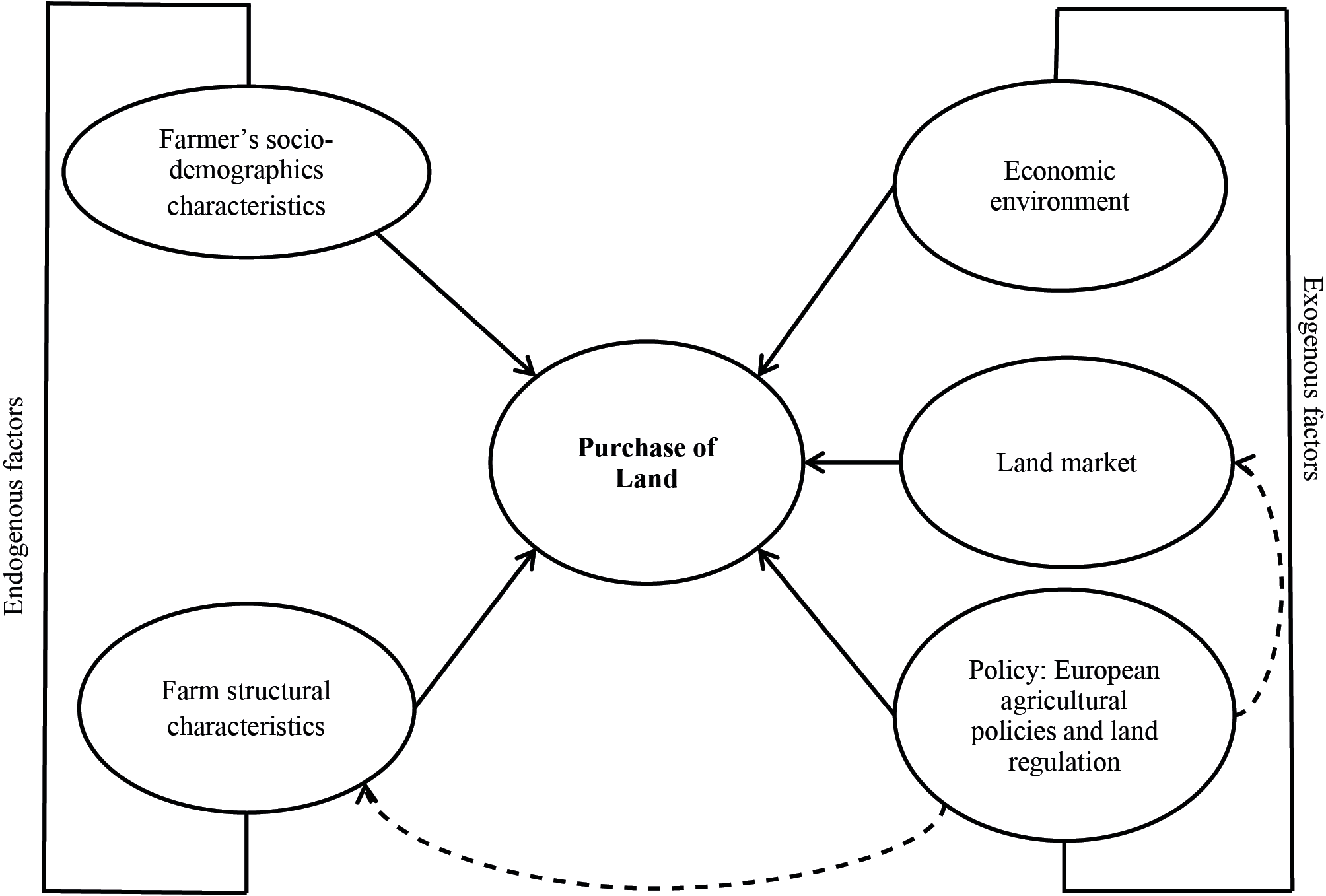
Based on the literature review, factors endogenous and exogenous to the farm that may have an influence have been identified and summarised in a conceptual model shown in Figure 1. Similar to the studies on farm size growth (Zimmermann et al., 2009), we do not assume that the identified exogenous and endogenous factors are independent of each other, but that they interact and condition each other.
3.1. Data and descriptive analysis
The analysis was conducted on Italian FADN data of Italian farms observed between 2013 and 2020. The data represent an unbalanced panel data consisting of 84610 observations representing 24212 farms. On average, the same farm remains in the sample for about 3 to 4 years.
For each farm, there is information on the structural characteristics of the farm, data on the farm’s balance sheet, and data on the socio-demographic characteristics of the farms.
Of the 24212 farms in the sample, 919 made at least one investment in land during the period in question, of these 176 farms made more than one investment (Table 1).
| Full Sample | Buyer | % | |
|---|---|---|---|
| Number of observations | 84610 | 1095 | 1.3 |
| Number of farms | 24212 | 919 | 3.8 |
Around 90% of the sample is characterised by specialised farms in cereals, arable crops, horticulture, fruit crops, olive growing, viticulture, dairy cattle, herbivores and granivores. The remaining 9.45% by non-specialised farms, of which 9.4% are mixed crop and livestock farms. Thirty-two percent of the sample is specialised in annual crops, 29.9% are permanent crops and 27.8% livestock farms (Table 2). Thirty-nine percent of the land purchases were conducted by farms specialising in permanent crops, followed by farms specialising in annual crops and livestock. In particular, 18% of the recorded transactions were conducted by farms specialising in fruit crops, 16.5% by vineyards, and 12% by farms specialising in arable crops (Table 2).
| Specialization | Sample | % Total observation | Buyers | % Total observation |
|---|---|---|---|---|
| N. Observations | N. Observations | |||
| No specialisation: | 7997 | 9.45 | 91 | 8.3 |
| Unclassifiable farms | 11 | 0.013 | 0 | 0 |
| Mixed crops and livestock farming | 7986 | 9.4 | 91 | 8.3 |
| Annual Crops | 27796 | 32.9 | 312 | 28.5 |
| Cereals | 8812 | 10.4 | 102 | 9.3 |
| Arable Crops | 10292 | 12.2 | 133 | 12.15 |
| Horticulture | 8692 | 10.3 | 77 | 7.03 |
| Permanent Crops | 25305 | 29.9 | 432 | 39.45 |
| Fruit Crops | 10721 | 12.7 | 202 | 18.45 |
| Olive growing | 4034 | 4.8 | 47 | 4.3 |
| Viticulture | 10550 | 12.5 | 183 | 16.7 |
| Livestock farms | 23512 | 27.8 | 260 | 23.75 |
| Dairy cattle | 7339 | 8.7 | 102 | 9.3 |
| Herbivores | 12108 | 14.3 | 102 | 9.3 |
| Granivores | 4065 | 4.8 | 56 | 5.1 |
| TOT | 84610 | 100 | 1095 | 100 |
In terms of average UAA, specialised livestock farms are the largest, followed by annual crops and permanent crops. Among all specialisations, farms specialised in viticulture have the smallest average farm size followed by those specialised in fruit crops and horticulture. There is an important difference in farm size between horticultural farms and those specialised in other annual crops. Farms specialised in permanent crops have lower “RENT/UAA” ratios than farms specialised in annual crops and livestock (Appendix 1).
Since the investment decision represents a discrete problem (Elhorst, 1993), to estimate the probability of participation decision we adopted a probit regression model.
The empirical model implemented to conduct the quantitative analysis was developed based on the conceptual model in figure 1 and peculiarities of FADN data. In particular, the characteristics of our database did not allow us to conduct a dynamic analysis, which would be appropriate since investments in capital stock are not annual investments (Lefebvre et al., 2015) and generally do not occur at the same time as they are planned (Elhorst, 1993).
The empirical probit model used is described by the following equation:
Where:
y*i is the binary dependent variable that assumes a value equal to 1 in the year in which the purchase occurs, 0 otherwise.
εi is the composite error term.
i represents the single observation,
xki is the observed value of explanatory variables that described factors linked to farm characteristics, farmer socio-demographic characteristics and exogenous variables.
The effect of xi on is represented by . and are respectively the intercept and the errors for i.
The equation is estimated using the ‘glm’ function in Rstudio of the ‘stats’ package.
The explanatory variables (Table 3) introduced in the probit model are listed and defined below.
| Variables | Specification | Type of variable | Expected effect |
|---|---|---|---|
| Farm structural characteristics | |||
| UAAsq | Utilised Agricultural Area square | Continuous | + |
| Production specialisation | Agricultural specialisations considered are: cereals, arable crops, horticulture, fruit crops, olive growing, viticulture, dairy cattle, herbivores, granivores. | Categorical; Non-specialised farms as reference |
+ |
| VA/ha | Ratio between Value added (excluding Income subsidies and COM subsidies) and UAA | Continuous | + |
| VA/ TWU | Ratio between Value Added and total work units | Continuous | + |
| UAASQ *Production Specialisation | Continuous*categorical; non-specialised farms as reference | + | |
| VA/ha*Specialisation | Continuous*categorical; Non-Specialised farms as reference |
+ | |
| VA/TWU*Specialisation | Continuous*categorical; Non-Specialised farms as reference |
+ | |
| RENT/UAA | The ratio of the rented UAA to the UAA | Continuous | +/- |
| Machinery_ Plant value | Value of Machinery+ equipment + plant; It represents a proxy variable for level of innovation on farms | Continuous | + |
| Income subsidies/ha | Aid per hectare provided by First Pillar and COM | Continuous | + |
| Investment subsidy | Investment aid (Second Pillar) | Continuous | + |
| Energy Production | Farm produces renewable energy | Dummy | + |
| Subcontracting activities | Farm carries subcontracting activities | Dummy | + |
| Agrotourism | Farm carries out agrotourism activities | Dummy | + |
| Pre_purchase | Purchases made between 2010-2020 | Dummy | + |
| FWU/TWU | Ratio of family work units to total work units | Continuous | + |
| Farmer sociodemographic characteristics | |||
| FARMER_18_39 | The farm manager is between 18 and 39 years old | Dummy | + |
| FARMER_40_49 | The farm manager is between 40 and 49 years old | Dummy | + |
| FARMER_50_59 | The farm manager is between 50 and 59 years old | Dummy | - |
| FARMER_OVER60 | The farm manager is aged 60 old or older | Dummy | - |
| SUCC_1_39 | There is a potential successor aged between 1 and 39 on the farm | Dummy | + |
| OFFFARM_INCOME | Farmer with non-agricultural income >2,000 euro; Children/grandchildren, father-in-law, parent, wife employed part-time or regularly with non-agricultural income >2000 euro | Dummy | + |
| Exogenous variables | |||
| INTEREST RATE | Interest rate recorded for each year on the Ministry of the Treasury website | Continuous | + |
| INFLATION_ RATE | Inflation rate taken for each year from the ISTAT website | Continuous | - |
3.2.1. Description of the explanatory variables and expected relation
Utilized agricultural area
It is unclear what effect the initial size of the farm may have on the growth of farm size and on the investment decision. Given the nature and characteristic of the data of this variable, it was decided to introduce as an explanatory variable the “UAA SQ” which represents the squared value of the total initial UAA of the farm regardless of whether it is owned, leased, or free use. The use of the square variable is able to catch the non-linear effect of it. Assuming that farm size can also be a measure of the farm’s ability to generate income (Oude Lansink et al. 2001), we expect this variable to have a positive effect on the investment decision.
Value added per hectares
This variable was introduced as an explanatory variable representing the productivity of land. Through this variable, the aim is to understand whether the productivity per hectare derived from the farm’s activity affects the growth of the farm size through purchase. According to the literature, the farmer is encouraged to buy land when productivity is high (Ciaian et al., 2010). Therefore, it is assumed that, as productivity per hectare increases, the likelihood of the farmer investing in land increases.
Value added per total work unit
This explanatory variable represents the productivity of farm labour. It is defined as the ratio of value added to total work units. It is assumed that as productivity per labour unit increases, the probability of the farmer purchasing land also increases.
Production Specialisation
When not focusing on a single specialization (e.g., the dairy sector), the researchers introduced a categorical variable related to farm specialisation (e.g Akimowicz et al., 2013) in order to understand whether the type of farm could influence the farm growth or investment decision. This is probably related to the fact that the type of assets needed by a farm varies according to their specialisation (Lefebvre et al., 2015). The data at our disposal include specialised and non-specialised farms. Specialisation is defined according to the technical-economic orientation of the FADN database (FADN, 2018). In contrast to this original classification, in this model farms classified as “mixed crop and livestock” are included in the “non-specialised farms”. Specialised farms fall into 9 categories: Cereal crops, arable crops, horticulture, fruit crops, olive crops, viticulture, dairy cattle, herbivores and granivores. Therefore, the explanatory variable was introduced into the model to account for the nine specialisation categories. “No specialisation” is used as the reference category since specialisation is one of the main drivers of the search for economies of scale and farm growth. Introducing this variable allows us to understand not only whether specialised farms invest more than non-specialised ones, but also whether the probability of buying land in Italy changes as specialisation changes.
Utilised agricultural area *Specialisation
The necessary assets of a farm and the “optimal size” vary depending on the type of farming (Lefebvre et al., 2015; Plogmann et al., 2022). In order to test whether the effect of farm size can vary according to the type of farming, it was decided to combine the two previous variables “UAAsq” and “Specialisation”., (Bremmer and Oude Lansink, 2002).
Rent/Utilised agricultural area
On the one hand, renting allows the farm more flexibility and the possibility to invest its liquidity in other productive assets (Swinnen et al., 2016). On the other hand, land managed as property allows the farmer to use it as collateral capital and thus to have greater access to credit (Swinnen et al., 2016). It was decided to introduce the ratio of the land managed under rent to the total utilised agricultural area of the farm as an inverse measure of the amount of collateral available (Benjamin and Phimister, 2002; Lefebvre et al., 2015). However, expectations on the direction of the effects of this variable are ambiguous.
Machinery Plant Value
Machinery and plant represent another form of collateral capital for a farm. It is assumed that high values of this variable correspond to a farm’s recent investment in such productive assets that vary proportionally to the farm area (Plogmann et al., 2022). Furthermore, there is a correlation between the intention to purchase land and investment in other farm assets (Lefebvre et al., 2015).Therefore, it is hypothesised that the farm is inclined to purchase with the aim of maximising the productive capacity of the asset in which it has previously invested.
Common Agricultural Policy
The Common Agricultural Policy has been identified as an exogenous factor that can influence the land price, but also the decision and level of investment. Subsidies received and capital financing are not the same for every farm and for this reason it can be considered as an endogenous variable linked to structural characteristics of the farm. It was decided to introduce two continuous variables. the first, the ratio of income subsidies per hectare related to the first pillar of the Common Agricultural Policy and COM. The second, the value of the investment subsidies received by the farm between 2013 and 2020 and connected to the measures of the second pillar of the Common Agricultural Policy.
Pre-purchase
Investment in land is a planned, long-term investment (Elhorst, 1993; Oskam et al., 2009; Oude Lansink et al., 2001). The land market is thin and local, and it could be difficult for a farmer to find the amount of land he wants at one time. (Cotteleer et al., 2008; Elhorst, 1993). Therefore, it may happen that the farmer must make more than one purchase to reach the desired level of investment. The dummy variable “Pre_Purchase” assumes a value equal to one when the purchasing farm has already made a purchase previously between 2011 and 2020.
Diversification activities
In the literature reviewed, researchers have not considered the role that farm-related activities can have on farm growth and the investment decision. The related activities that can be stimulated by RDP measures allow for a diversification of the farm activity and represent a different form of income for the agricultural firm. Three dummy variables were introduced for three agricultural related activities: agrotourism, energy production and contracting. It is expected that conducting agricultural related activities increases the probability that the purchase will occur.
Family work units
Family labour can be considered as a fixed input of production within the farm (Elhorst, 1993) and Elhorst’s research showed that as family labour input increases, investment increases. Weiss (1999) and Oude Lansink et al. (2001) showed that the number of family members affects farm growth and the investment decision. The variable FWU/TWU was introduced into the model as a measure of how much the business depends on family labour. It is hypothesised that family farms have a greater interest in investing in the farm and farm growth and thus, as this ratio increases, the probability that the farm invests in land increases.
Age of farmer and successor
The age of the farmer and the presence of the successor can affect the growth of the farm and the investment decision. Since there may be several farmers and potential successors with different ages on the same farm, it was decided to create four dummy variables related to the holder and his/her age, and one related to the presence of the successor. In particular, four age ranges were identified to which dummy variables corresponded. Each dummy variable relating to the holder takes the value of one if there are no successors for that observation and if the holder or all the holders fall within the range defined by the dummy variable. If the observation corresponds to more than one holder falling in different age groups, all variables related to the holders will have value zero. The variable relating to the presence of a successor will take a value of 1 if there is at least one potential successor between the ages of 1 year and 40 years. A successor was the one who was classified within the dataset as the ‘son’ or ‘grandson’ of the farmer.
Off-farm income
In the literature, it is unclear whether the earning of an off-farm income can be a prelude to leaving the sector or represents a form of income that allows the farm to survive better and not leave the sector (Lefebvre et al., 2015; Plogmann et al., 2022). Based on the available data, a dummy variable was created which takes the value of 1 if the farmer or a member of his or her family who is employed part-time or full-time on the farm earns an off-farm income >2000 euros.
As mentioned before, land is considered an asset that can be used as collateral and a safe investment option. The model introduces two external factors: inflation rate and interest rate. It is assumed that when inflation rates rise, the likelihood of purchasing land also increases. However, buying land may require a significant investment that the farm may need to finance through a bank loan. As interest rates go up, the probability of making such an investment decrease. The inflation rate values, Consumer Price Index-CPI, are obtained from the ISTAT website every December of the reference year, while the interest rate is determined by the average annual yield of Italian BTPs (Multi-year Treasury Bonds), which can be found on the website of the Italian Treasury Ministry.
3.2.3. Descriptive analysis of explanatory variables
Table 4 shows the descriptive analysis of the variables included in the model, in particular each variable has two values: one for all farms and one for “buyers” (farms investing in land during the reference period). The average initial area of the sample is 33.7 ha, which increases by about 5 ha if only buyers are taken into account. The value related to value added per hectare (VA/ha) exhibits significant variations among the farms. Nevertheless, these differences decrease considerably when only the buyers are considered. Furthermore, the average value of the variable “VA/ha” is lower for the buyers, whereas the median value for buyers is higher than the value within the entire sample. The average value of machinery and plant of the farms that invested in land is more than twice as high as the sample average. There are also important differences in both the median value and the standard deviation. For the ratio of rented area to total farm area and of family labour units to total farm hours, there are no important differences between the farms that purchase and the entire sample. It should be noted that the purchasing farms have on average lower FWU/TWU than the sample farms. The sample farms received, on average, a higher subsidy/hectare and capital financing than the buying farms. Analysing the value of the median and standard deviation of the variable for subsidies/ha related to the first pillar, the farms received a higher subsidy and a greater dispersion of values around the mean. For the period taken into account, there are no important differences in the variables related to the exogenous context.
| Variable | Min | Mean | Median | Standard Deviation | Max |
|---|---|---|---|---|---|
| Farm structural characteristics | |||||
| UAA | 0.01 | 33.72 | 15.1 | 57.7 | 1754 |
| UAA_BUYER | 0.23 | 37.73 | 19.54 | 62.17 | 909.75 |
| UAAsq | 0 | 4467.1 | 227.9 | 32704.46 | 3076516.0 |
| UAAsq_BUYER | 0.1 | 5286 | 381.8 | 35908.68 | 827645 |
| VA/ha | -209342 | 7121 | 2108 | 32496.66 | 3792972 |
| VA/ha_BUYER | -2711 | 6345 | 3027 | 10541.81 | 117597 |
| VA/TWU | -838045 | 35197 | 25057 | 38215.14 | 1069950 |
| VA/TWU_BUYER | -18615 | 43418 | 32776 | 43381.17 | 468484 |
| Machinery and Plant Value | -1628809 | 34683 | 6310 | 114923.9 | 5450764 |
| Machineryand Plant Value_BUYER | 0 | 79280 | 30239 | 210057.8 | 4900435 |
| Rent/UAA | 0 | 0.38 | 0.19 | 0.41 | 1 |
| Rent/UAA_BUYER | 0 | 0.3446 | 0.1954 | 0.3785 | 1 |
| Income Subsidies/ha | 0 | 260.1 | 373.8 | 1071.23 | 121033.9 |
| Income Subsidies/ha_Buyer | 0 | 386.4 | 273.6 | 510.5 | 6408 |
| Investment subsidy | 0 | 583.9 | 0 | 6.866.118 | 639170 |
| Capital Account_Buyer | 0 | 2008 | 0 | 15679 | 435000 |
| Energy production | 0 | 0.3679 | 0 | 0.18816 | 1 |
| Energy production_ Buyer | 0 | 0.075 | 0 | 0.264 | 1 |
| Subcontracting activities | 0 | 0.03543 | 0 | 0.1848 | 1 |
| Subcontracting activities_buyer | 0 | 0.064 | 0 | 0.246 | 1 |
| Agroturism | 0 | 0.04306 | 0 | 0.20298 | 1 |
| Agroturism_ buyer | 0 | 0.05 | 0 | 0.218 | 1 |
| Pre_Purchase | 0 | 0.0026 | 0 | 0.051 | 1 |
| Pre_Purchase_Buyer | 0 | 0.2 | 0 | 0.4 | 1 |
| FWU/TWU | 0 | 0.837 | 1 | 0.25 | 1 |
| FWU/TWU_Buyer | 0.017 | 0.75 | 0.92 | 0.29 | 1 |
| Farmer sociodemographic characteristics | |||||
| 18≤FARMER≤39 | 0 | 0.14 | 0 | 0.35 | 1 |
| 18≤FARMER≤39_ Buyer | 0 | 0.17 | 0 | 0.38 | 1 |
| 40≤FARMER≤49 | 0 | 0.21 | 0 | 0.41 | 1 |
| 40≤FARMER≤49_ Buyer | 0 | 0.25 | 0 | 0.43 | 1 |
| 50≤FARMER≤59 | 0 | 0.23 | 0 | 0.42 | 1 |
| 50≤FARMER≤59_ Buyer | 0 | 0.22 | 0 | 0.41 | 1 |
| FARMER>60 | 0 | 0.28 | 0 | 0.45 | 1 |
| FARMER>60_Buyer | 0 | 0.16 | 0 | 0.37 | 1 |
| 1≤SUCCESSOR≤39 | 0 | 0.09 | 0 | 0.29 | 1 |
| 1≤SUCCESSOR≤39_ Buyer | 0 | 0.13 | 0 | 0.34 | 1 |
| OFF_FARM INCOME | 0 | 0.16 | 0 | 0.36 | 1 |
| OFF_FARM INCOME_Buyer | 0 | 0.24 | 0 | 0.43 | 1 |
| Exogenous factors | |||||
| Inflation rate | -0.20 | 0.45 | 0.5 | 0.42 | 1.1 |
| Interest rate | 1.14 | 1.86 | 1.81 | 0.77 | 3.6 |
To the best of our knowledge, there is no research of this type in the literature. Therefore, it was decided to run five probit regression models to better understand how different factors might influence the land investment decision:
– Model 1: the model considers all the variables described above and summarised in Table 5 except for the variables “VA/ha” and “VA/TWU”. Thus, the model only considers the “UAAsq” as the farm size variable.
– Model 2: Same as previous model, but the variable “UAAsq” also interacts with specialisation (“UAAsq* Specialisation”).
– Model 3: to model 1, the two variables farm productivity per ha (VA/ha) and farm productivity per total work unit (VA/TWU) were included.
– Model4: same as model 3 adding an interaction between the variable “Specialization” and the two variables “UAAsq” and “VA/ha” (“UUAsq* Specialisation”, and “VA/ha*Specialisation”).
– Model 5: same as model 3 but the “UAAsq”, “VA/ha” and VA/TWU variables interact with the specialisation variable.
4.1. Correlation analysis and VIF analysis
To verify that there is no relationship among the independent variables, a Pearson correlation analysis and Variance Inflation factors (VIF) were conducted. The results (Appendix 2) show that the indices between the independent variables are far from the threshold values. Thus, it can be ruled out that there is multicollinearity between the variables considered in the empirical model developed.
The five implemented models (Tables 5, 6, 7, 8, 9) explain between 19 and 20% of the land investment decision of the observed farms between 2013 and 2020. Even adding the two variables “VA/ha” and “VA/TWU” and the interaction of the variable “Specialisation” with “UAAsq”, “VA/ ha”, and “VA/TWU” did not improve the model. As the intercept value also shows, there are other factors that were not considered that influenced the purchase decision. In addition to the value of Pseudo R2 not varying, the sign of the independent variables also never changes in the different models implemented. This indicates a good level of robustness of the model.
| Variable | Estimate | Std.error | Statistic | p. value | |||||||||||||||
|---|---|---|---|---|---|---|---|---|---|---|---|---|---|---|---|---|---|---|---|
| (Intercept) | -2.02925 | 0.104478 | -19.4227 | 4.96E-84 | *** | ||||||||||||||
| Farm structural characteristics | |||||||||||||||||||
| UAASq | -1.2E-06 | 7.1E-07 | -1.72448 | 0.084622 | . | ||||||||||||||
| No specialisation | |||||||||||||||||||
| Cereals | 0.050576 | 0.061861 | 0.817562 | 0.413607 | |||||||||||||||
| Arable Crops | 0.055266 | 0.05832 | 0.947622 | 0.343322 | |||||||||||||||
| Horticulture | -0.13114 | 0.065892 | -1.99019 | 0.04657 | * | ||||||||||||||
| Fruit Crops | 0.127162 | 0.055627 | 2.285978 | 0.022256 | * | ||||||||||||||
| Olive growing | -0.01181 | 0.074624 | -0.15824 | 0.87427 | |||||||||||||||
| Viticulture | 0.124953 | 0.055829 | 2.238162 | 0.025211 | * | ||||||||||||||
| Dairy cattle | 0.039657 | 0.062406 | 0.635463 | 0.525127 | |||||||||||||||
| Herbivores | -0.04975 | 0.05958 | -0.835 | 0.403718 | |||||||||||||||
| Granivores | 0.014759 | 0.074215 | 0.198868 | 0.842366 | |||||||||||||||
| RENT/UAA | -0.1214 | 0.033698 | -3.60269 | 0.000315 | *** | ||||||||||||||
| FWU/TWU | -0.33055 | 0.049356 | -6.69724 | 2.12E-11 | *** | ||||||||||||||
| Machinary_ Plant Value | 3.19E-07 | 7.02E-08 | 4.539024 | 5.65E-06 | *** | ||||||||||||||
| Subsidies UE/SAU` | 1.9E-06 | 1.06E-05 | 0.179035 | 0.85791 | |||||||||||||||
| Capital Account | 1.74E-06 | 1.09E-06 | 1.585145 | 0.112933 | |||||||||||||||
| Energy production | 0.145373 | 0.05958 | 2.439938 | 0.01469 | * | ||||||||||||||
| Subcontracting activities | 0.211659 | 0.058079 | 3.644351 | 0.000268 | *** | ||||||||||||||
| Agrotourism | -0.03798 | 0.061303 | -0.61953 | 0.53557 | |||||||||||||||
| Pre_PURCHASE | 7.473506 | 24.51225 | 0.304889 | 0.760451 | |||||||||||||||
| Farm socio-demographic characteristics | |||||||||||||||||||
| FARMER_18_39 | 0.223549 | 0.080916 | 2.762715 | 0.005732 | ** | ||||||||||||||
| FARMER_40_49 | 0.176139 | 0.078891 | 2.23268 | 0.02557 | * | ||||||||||||||
| FARMER_50_59 | 0.102417 | 0.079003 | 1.296358 | 0.194852 | |||||||||||||||
| FARMER_OVER60 | -0.04849 | 0.079899 | -0.60692 | 0.543907 | |||||||||||||||
| SUCC_1_39 | 0.210418 | 0.082712 | 2.543965 | 0.01096 | * | ||||||||||||||
| OFF_FARM INCOME | 0.116554 | 0.032475 | 3.58899 | 0.000332 | *** | ||||||||||||||
| Exogenous factors | |||||||||||||||||||
| Inflation rate | 0.102711 | 0.031766 | 3.233331 | 0.001224 | ** | ||||||||||||||
| Interest rate | -0.12116 | 0.020088 | -6.03132 | 1.63E-09 | *** | ||||||||||||||
| N. observations | 84610 | ||||||||||||||||||
| N. farms | 24212 | ||||||||||||||||||
| Pseudo R2 | 0.1969 | ||||||||||||||||||
| AIC | 9449.1 | ||||||||||||||||||
| Signif. codes: 0 ‘***’ 0.001 ‘**’ 0.01 ‘*’ 0.05 ‘.’ 0.1 ‘ ’ 1. | |||||||||||||||||||
| Variable | Estimate | Std.error | Statistic | p. value | |||||||||||||||
|---|---|---|---|---|---|---|---|---|---|---|---|---|---|---|---|---|---|---|---|
| (Intercept) | -1.97278 | 0.106974 | -18.4418 | 6.07E-76 | *** | ||||||||||||||
| Farm structural characteristics | |||||||||||||||||||
| UAASq | -1.8E-05 | 1.01E-05 | -1.76454 | 0.077641 | . | ||||||||||||||
| No specialisation | *ref. | ||||||||||||||||||
| Cereals | 0.014812 | 0.065264 | 0.226955 | 0.820458 | |||||||||||||||
| Arable Crops | 0.035546 | 0.061341 | 0.579489 | 0.562259 | |||||||||||||||
| Horticulture | -0.17526 | 0.068388 | -2.56278 | 0.010384 | * | ||||||||||||||
| Fruit Crops | 0.080197 | 0.058392 | 1.373422 | 0.169621 | |||||||||||||||
| Olive growing | -0.01889 | 0.079616 | -0.2372 | 0.812499 | |||||||||||||||
| Viticulture | 0.081881 | 0.058412 | 1.401778 | 0.160982 | |||||||||||||||
| Dairy cattle | 0.016336 | 0.066267 | 0.246521 | 0.805279 | |||||||||||||||
| Herbivores | -0.09526 | 0.062141 | -1.53296 | 0.125286 | |||||||||||||||
| Granivores | 0.009716 | 0.078393 | 0.123935 | 0.901367 | |||||||||||||||
| UAAsq*No specialisation | *ref. | ||||||||||||||||||
| UAAsq*Cereals | 1.63E-05 | 1.02E-05 | 1.591816 | 0.111426 | |||||||||||||||
| UAA sq*Arable Crops | 1.2E-05 | 1.05E-05 | 1.144364 | 0.252473 | |||||||||||||||
| UAA sq*Horticulture | 1.8E-05 | 1.02E-05 | 1.76043 | 0.078335 | . | ||||||||||||||
| UAA sq*Fruit Crops | 2.21E-05 | 1.06E-05 | 2.090571 | 0.036567 | * | ||||||||||||||
| UAA sq*Olive growing | -2.8E-05 | 4.34E-05 | -0.64604 | 0.518253 | |||||||||||||||
| UAA sq*Viticulture | 2.01E-05 | 1.05E-05 | 1.913096 | 0.055736 | . | ||||||||||||||
| UAA sq*Dairy cattle | 1.36E-05 | 1.05E-05 | 1.304731 | 0.191985 | |||||||||||||||
| UAA sq*Herbivores | 1.72E-05 | 1.01E-05 | 1.705913 | 0.088024 | . | ||||||||||||||
| UAA sq*Granivores | -1.1E-06 | 1.61E-05 | -0.06829 | 0.945555 | |||||||||||||||
| RENT/UAA | -0.11873 | 0.033778 | -3.51498 | 0.00044 | *** | ||||||||||||||
| FWU/TWU | -0.34668 | 0.050258 | -6.8979 | 5.28E-12 | *** | ||||||||||||||
| Machinary_ Plant Value | 3.59E-07 | 7.3E-08 | 4.916479 | 8.81E-07 | *** | ||||||||||||||
| Subsidies EU/SAU` | 1.19E-06 | 1.1E-05 | 0.107778 | 0.914172 | |||||||||||||||
| Capital Account | 1.66E-06 | 1.1E-06 | 1.50566 | 0.132155 | |||||||||||||||
| Energy production | 0.154468 | 0.059736 | 2.58584 | 0.009714 | ** | ||||||||||||||
| Subcontracting activities | 0.217539 | 0.058278 | 3.732783 | 0.000189 | *** | ||||||||||||||
| Agrotourism | -0.04088 | 0.061488 | -0.66492 | 0.506102 | |||||||||||||||
| Pre_PURCHASE | 12.8663 | 40.68004 | 0.316281 | 0.75179 | |||||||||||||||
| Farm socio-demographic characteristics | |||||||||||||||||||
| FARMER_18_39 | 0.21479 | 0.081078 | 2.64919 | 0.008068 | ** | ||||||||||||||
| FARMER_40_49 | 0.17053 | 0.079045 | 2.157388 | 0.030975 | * | ||||||||||||||
| FARMER_50_59 | 0.09462 | 0.079167 | 1.195197 | 0.23201 | |||||||||||||||
| FARMER_OVER60 | -0.05634 | 0.080087 | -0.70349 | 0.481748 | |||||||||||||||
| SUCC_1_39 | 0.20331 | 0.082879 | 2.453102 | 0.014163 | * | ||||||||||||||
| OFF_FARM INCOME | 0.116426 | 0.032544 | 3.577474 | 0.000347 | *** | ||||||||||||||
| Exogenous factors | |||||||||||||||||||
| Inflation rate | 0.103918 | 0.031817 | 3.266172 | 0.00109 | ** | ||||||||||||||
| Interest rate | -0.12202 | 0.020131 | -6.06119 | 1.35E-09 | *** | ||||||||||||||
| N. observations | 84610 | ||||||||||||||||||
| N. farms | 24212 | ||||||||||||||||||
| Pseudo R2 | 9446.3 | ||||||||||||||||||
| AIC | 0.1986 | ||||||||||||||||||
| Signif. codes: 0 ‘***’ 0.001 ‘**’ 0.01 ‘*’ 0.05 ‘.’ 0.1 ‘ ’ 1. | |||||||||||||||||||
| Variable | Estimate | Std.error | Statistic | p. value | |||||||||||||||
|---|---|---|---|---|---|---|---|---|---|---|---|---|---|---|---|---|---|---|---|
| (Intercept) | -2.045 | 0.105 | -19.397 | 8.18E-84 | *** | ||||||||||||||
| Farm structural characteristics | |||||||||||||||||||
| UAASq | -1.5E-06 | 7.7E-07 | -2.00308 | 0.0451687 | * | ||||||||||||||
| AV/ha | -1.6E-06 | 9.46E-07 | -1.7294 | 0.08373801 | . | ||||||||||||||
| AV/TWU | 8.63E-07 | 3.3E-07 | 2.616924 | 0.0088726 | ** | ||||||||||||||
| No specialisation | *ref. | ||||||||||||||||||
| Cereals | 0.037215 | 0.062066 | 0.599605 | 0.54876961 | |||||||||||||||
| Arable Crops | 0.050264 | 0.058365 | 0.861204 | 0.38912569 | |||||||||||||||
| Horticulture | -0.10695 | 0.067537 | -1.5835 | 0.11330853 | |||||||||||||||
| Fruit Crops | 0.128527 | 0.055697 | 2.307599 | 0.02102146 | * | ||||||||||||||
| Olive growing | -0.01248 | 0.074735 | -0.16703 | 0.86734686 | |||||||||||||||
| Viticulture | 0.122659 | 0.056015 | 2.189751 | 0.02854231 | * | ||||||||||||||
| Dairy cattle | 0.025609 | 0.062677 | 0.408584 | 0.68284533 | |||||||||||||||
| Herbivores | -0.05549 | 0.05965 | -0.93024 | 0.35224614 | |||||||||||||||
| Granivores | 0.001192 | 0.076438 | 0.015592 | 0.9875601 | |||||||||||||||
| RENT/UAA | -0.12716 | 0.033848 | -3.75693 | 0.00017201 | *** | ||||||||||||||
| FWU/TWU | -0.33126 | 0.049916 | -6.63638 | 3.2148E-11 | *** | ||||||||||||||
| Machinary_ Plant Value | 2.8E-07 | 7.26E-08 | 3.856252 | 0.00011514 | *** | ||||||||||||||
| Subsidies UE/SAU` | 2.34E-06 | 1.18E-05 | 0.197617 | 0.84334507 | |||||||||||||||
| Capital Account | 1.77E-06 | 1.09E-06 | 1.620226 | 0.10518384 | |||||||||||||||
| Energy production | 0.135872 | 0.059832 | 2.270884 | 0.023154 | * | ||||||||||||||
| Subcontracting activities | 0.207201 | 0.058176 | 3.561636 | 0.00036855 | *** | ||||||||||||||
| Agrotourism | -0.03057 | 0.061388 | -0.49806 | 0.6184439 | |||||||||||||||
| Pre_PURCHASE | 7.463387 | 24.52 | 0.30438 | 0.76083871 | |||||||||||||||
| Farm socio-demographic characteristics | |||||||||||||||||||
| FARMER_18_39 | 0.223439 | 0.080945 | 2.760367 | 0.00577364 | * | ||||||||||||||
| FARMER_40_49 | 0.173963 | 0.078917 | 2.204384 | 0.02749733 | * | ||||||||||||||
| FARMER_50_59 | 0.100882 | 0.079033 | 1.27645 | 0.20179632 | |||||||||||||||
| FARMER_OVER60 | -0.04797 | 0.079945 | -0.60002 | 0.54849104 | |||||||||||||||
| SUCC_1_39 | 0.212866 | 0.082742 | 2.572654 | 0.01009221 | * | ||||||||||||||
| OFF_FARM INCOME | 0.120334 | 0.03258 | 3.693551 | 0.00022114 | *** | ||||||||||||||
| Exogenous factors | |||||||||||||||||||
| Inflation rate | 0.101524 | 0.031788 | 3.193758 | 0.00140434 | ** | ||||||||||||||
| Interest rate | -0.11983 | 0.02009 | -5.96484 | 2.4488E-09 | *** | ||||||||||||||
| N. observations | |||||||||||||||||||
| N. farms | |||||||||||||||||||
| Pseudo R2 | 0.197 | ||||||||||||||||||
| AIC | 9444.2 | ||||||||||||||||||
| Signif. codes: 0 ‘***’ 0.001 ‘**’ 0.01 ‘*’ 0.05 ‘.’ 0.1 ‘ ’ 1. | |||||||||||||||||||
| Variable | Estimate | Std.error | Statistic | p. value | |||||||||||||||
|---|---|---|---|---|---|---|---|---|---|---|---|---|---|---|---|---|---|---|---|
| (Intercept) | -1.99374 | 0.108933 | -18.3024 | 7.92E-75 | *** | ||||||||||||||
| Farm structural characteristics | |||||||||||||||||||
| UAASq | -1.9E-05 | 1.04E-05 | -1.85328 | 0.063842 | . | ||||||||||||||
| AV/ha | -7.1E-07 | 2.63E-06 | -0.2676 | 0.789008 | |||||||||||||||
| AV/TWU | 1E-06 | 3.51E-07 | 2.855578 | 0.004296 | ** | ||||||||||||||
| No specialisation | *ref. | ||||||||||||||||||
| Cereals | 0.072043 | 0.083218 | 0.865717 | 0.386645 | |||||||||||||||
| Arable Crops | 0.055166 | 0.066467 | 0.829975 | 0.406553 | |||||||||||||||
| Horticulture | -0.10531 | 0.077387 | -1.36083 | 0.173566 | |||||||||||||||
| Fruit Crops | 0.007115 | 0.065407 | 0.108785 | 0.913373 | |||||||||||||||
| Olive growing | 0.068962 | 0.10743 | 0.641925 | 0.520922 | |||||||||||||||
| Viticulture | 0.056009 | 0.063879 | 0.876809 | 0.380591 | |||||||||||||||
| Dairy cattle | 0.000847 | 0.077215 | 0.010964 | 0.991252 | |||||||||||||||
| Herbivores | -0.08485 | 0.065411 | -1.29714 | 0.194583 | |||||||||||||||
| Granivores | 0.007139 | 0.086704 | 0.082343 | 0.934374 | |||||||||||||||
| UAAsq*No specialisation | *ref. | ||||||||||||||||||
| UAAsq*Cereals | 1.75E-05 | 1.06E-05 | 1.649353 | 0.099075 | . | ||||||||||||||
| UAA sq*Arable Crops | 1.24E-05 | 1.1E-05 | 1.134469 | 0.256598 | |||||||||||||||
| UAA sq*Horticulture | 1.9E-05 | 1.07E-05 | 1.76849 | 0.076979 | . | ||||||||||||||
| UAA sq*Fruit Crops | 2.42E-05 | 1.09E-05 | 2.223406 | 0.026188 | * | ||||||||||||||
| UAA sq*Olive growing | -3.5E-05 | 4.61E-05 | -0.75006 | 0.453221 | |||||||||||||||
| UAA sq*Viticulture | 2.14E-05 | 1.09E-05 | 1.967757 | 0.049096 | * | ||||||||||||||
| UAA sq*Dairy cattle | 1.5E-05 | 1.08E-05 | 1.39341 | 0.163496 | |||||||||||||||
| UAA sq*Herbivores | 1.86E-05 | 1.04E-05 | 1.781584 | 0.074817 | . | ||||||||||||||
| UAA sq*Granivores | -5.2E-06 | 1.74E-05 | -0.29753 | 0.76606 | |||||||||||||||
| VA/ha*No specialisation | *ref. | ||||||||||||||||||
| VA/ha*Cereals | -7.3E-05 | 5.29E-05 | -1.38756 | 0.165271 | |||||||||||||||
| VA/ha*Arable Crops | -1E-05 | 8.97E-06 | -1.12181 | 0.261942 | |||||||||||||||
| VA/ha*Horticulture | -3.7E-06 | 3.45E-06 | -1.08411 | 0.278315 | |||||||||||||||
| VA/ha*Fruit Crops | 8.52E-06 | 4.23E-06 | 2.01371 | 0.04404 | * | ||||||||||||||
| VA/ha*Olive growing | -3.4E-05 | 2.67E-05 | -1.26886 | 0.204491 | |||||||||||||||
| VA/ha*Viticulture | 2.22E-06 | 3.93E-06 | 0.564954 | 0.572105 | |||||||||||||||
| VA/ha*Dairy cattle | -1.6E-06 | 8.2E-06 | -0.19265 | 0.847235 | |||||||||||||||
| VA/ha*Herbivores | -1.1E-05 | 9.75E-06 | -1.13936 | 0.254554 | |||||||||||||||
| VA/ha*Granivores | -1.2E-06 | 3.17E-06 | -0.36899 | 0.712137 | |||||||||||||||
| RENT/UAA | -0.12428 | 0.034028 | -3.65222 | 0.00026 | *** | ||||||||||||||
| FWU/TWU | -0.3474 | 0.051617 | -6.73025 | 1.69E-11 | *** | ||||||||||||||
| Machinary_ Plant Value | 3.04E-07 | 7.6E-08 | 4.001466 | 6.3E-05 | *** | ||||||||||||||
| Subsidies UE/SAU` | 1.85E-05 | 1.72E-05 | 1.07629 | 0.281797 | |||||||||||||||
| Capital Account | 1.66E-06 | 1.11E-06 | 1.500508 | 0.133483 | |||||||||||||||
| Energy production | 0.147989 | 0.06 | 2.46649 | 0.013644 | * | ||||||||||||||
| Subcontracting activities | 0.214248 | 0.058618 | 3.654989 | 0.000257 | *** | ||||||||||||||
| Agrotourism | -0.04545 | 0.062279 | -0.72979 | 0.465517 | |||||||||||||||
| Pre_PURCHASE | 13.97034 | 39.52004 | 0.3535 | 0.723714 | |||||||||||||||
| Farm socio-demographic characteristics | |||||||||||||||||||
| FARMER_18_39 | 0.211627 | 0.081357 | 2.601209 | 0.00929 | ** | ||||||||||||||
| FARMER_40_49 | 0.166384 | 0.079334 | 2.097254 | 0.035971 | * | ||||||||||||||
| FARMER_50_59 | 0.090013 | 0.079462 | 1.132779 | 0.257307 | |||||||||||||||
| FARMER_OVER60 | -0.05757 | 0.08041 | -0.71592 | 0.474042 | |||||||||||||||
| SUCC_1_39 | 0.197505 | 0.083187 | 2.374226 | 0.017586 | * | ||||||||||||||
| OFF_FARM INCOME | 0.116606 | 0.03276 | 3.559429 | 0.000372 | *** | ||||||||||||||
| Exogenous factors | |||||||||||||||||||
| Inflation rate | 0.102362 | 0.031866 | 3.212269 | 0.001317 | ** | ||||||||||||||
| Interest rate | -0.12011 | 0.020178 | -5.95262 | 2.64E-09 | *** | ||||||||||||||
| N. observations | 84610 | ||||||||||||||||||
| N. farms | 24121 | ||||||||||||||||||
| Pseudo R2 | 0.2 | ||||||||||||||||||
| AIC | 9440 | ||||||||||||||||||
| Signif. codes: 0 ‘***’ 0.001 ‘**’ 0.01 ‘*’ 0.05 ‘.’ 0.1 ‘ ’ 1. | |||||||||||||||||||
| Variable | Estimate | Std.error | Statistic | p. value | |||||||||||||||
|---|---|---|---|---|---|---|---|---|---|---|---|---|---|---|---|---|---|---|---|
| (Intercept) | -1.99498 | 0.115489 | -17.2742 | 7.36E-67 | *** | ||||||||||||||
| Farm structural characteristics | |||||||||||||||||||
| UAASq | -2E-05 | 1.11E-05 | -1.81586 | 0.069391 | . | ||||||||||||||
| VA/ha | -7.9E-07 | 2.86E-06 | -0.27699 | 0.781788 | |||||||||||||||
| VA/TWU | 1.32E-06 | 1.65E-06 | 0.799903 | 0.423767 | |||||||||||||||
| No specialisation | |||||||||||||||||||
| Cereals | 0.07122 | 0.092882 | 0.766783 | 0.443211 | |||||||||||||||
| Arable Crops | 0.09771 | 0.082926 | 1.178278 | 0.238686 | |||||||||||||||
| Horticulture | -0.13821 | 0.097122 | -1.42309 | 0.15471 | |||||||||||||||
| Fruit Crops | 0.023628 | 0.081487 | 0.28996 | 0.771847 | |||||||||||||||
| Olive growing | 0.051554 | 0.121524 | 0.424233 | 0.671396 | |||||||||||||||
| Viticulture | 0.057211 | 0.077299 | 0.740133 | 0.459219 | |||||||||||||||
| Dairy cattle | 0.082709 | 0.093701 | 0.88269 | 0.377404 | |||||||||||||||
| Herbivores | -0.07159 | 0.080316 | -0.89129 | 0.372772 | |||||||||||||||
| Granivores | -0.03472 | 0.103522 | -0.33543 | 0.737302 | |||||||||||||||
| UAAsq*No specialisation | |||||||||||||||||||
| UAAsq*Cereals | 1.78E-05 | 1.13E-05 | 1.576344 | 0.114946 | |||||||||||||||
| UAA sq*Arable Crops | 1.49E-05 | 1.16E-05 | 1.281408 | 0.200051 | |||||||||||||||
| UAA sq*Horticulture | 1.92E-05 | 1.16E-05 | 1.644969 | 0.099976 | . | ||||||||||||||
| UAA sq*Fruit Crops | 2.51E-05 | 1.15E-05 | 2.170636 | 0.029959 | * | ||||||||||||||
| UAA sq*Olive growing | -4.5E-05 | 5.18E-05 | -0.86149 | 0.388966 | |||||||||||||||
| UAA sq*Viticulture | 2.2E-05 | 1.15E-05 | 1.912193 | 0.055851 | . | ||||||||||||||
| UAA sq*Dairy cattle | 1.7E-05 | 1.14E-05 | 1.488127 | 0.136717 | |||||||||||||||
| UAA sq*Herbivores | 1.94E-05 | 1.11E-05 | 1.747083 | 0.080623 | . | ||||||||||||||
| UAA sq*Granivores | -1.1E-05 | 1.95E-05 | -0.56654 | 0.571024 | |||||||||||||||
| VA/ha*No specialisation | |||||||||||||||||||
| VA/ha*Cereals | -8.6E-05 | 5.8E-05 | -1.48766 | 0.136839 | |||||||||||||||
| VA/ha*Arable Crops | -8E-06 | 8.82E-06 | -0.9121 | 0.361714 | |||||||||||||||
| VA/ha*Horticulture | -3.7E-06 | 3.63E-06 | -1.02881 | 0.303568 | |||||||||||||||
| VA/ha*Fruit Crops | 9.08E-06 | 4.61E-06 | 1.968187 | 0.049047 | * | ||||||||||||||
| VA/ha*Olive growing | -4.3E-05 | 3.07E-05 | -1.41899 | 0.155902 | |||||||||||||||
| VA/ha*Viticulture | 1.76E-06 | 4.38E-06 | 0.401473 | 0.688072 | |||||||||||||||
| VA/ha*Dairy cattle | 6.37E-06 | 8.45E-06 | 0.753606 | 0.451086 | |||||||||||||||
| VA/ha*Herbivores | -1.1E-05 | 1.02E-05 | -1.0554 | 0.291243 | |||||||||||||||
| VA/ha*Granivores | -1.8E-06 | 3.54E-06 | -0.50791 | 0.611519 | |||||||||||||||
| AV/TWU*No specialisation | |||||||||||||||||||
| AV/TWU*Cereals | 2.36E-07 | 2.02E-06 | 0.116892 | 0.906946 | |||||||||||||||
| AV/TWU*Arable Crops | -1.7E-06 | 2.09E-06 | -0.81922 | 0.412663 | |||||||||||||||
| AV/TWU*Horticulture | 7.66E-07 | 2.04E-06 | 0.375434 | 0.707337 | |||||||||||||||
| AV/TWU*Fruit Crops | -7.4E-07 | 2.09E-06 | -0.35518 | 0.722453 | |||||||||||||||
| AV/TWU*Olive growing | 2.06E-06 | 3.96E-06 | 0.519424 | 0.603465 | |||||||||||||||
| AV/TWU*Viticulture | -5.5E-08 | 1.86E-06 | -0.02988 | 0.976165 | |||||||||||||||
| AV/TWU*Dairy cattle | -2.7E-06 | 2.1E-06 | -1.29293 | 0.196035 | |||||||||||||||
| AV/TWU*Herbivores | -5.1E-07 | 1.9E-06 | -0.27174 | 0.785824 | |||||||||||||||
| AV/TWU*Granivores | 5.28E-07 | 1.79E-06 | 0.295245 | 0.767807 | |||||||||||||||
| RENT/UAA | -0.12308 | 0.034091 | -3.6102 | 0.000306 | *** | ||||||||||||||
| FWU/TWU | -0.35157 | 0.051736 | -6.79551 | 1.08E-11 | *** | ||||||||||||||
| Machinary_ Plant Value | 3.23E-07 | 7.85E-08 | 4.112943 | 3.91E-05 | *** | ||||||||||||||
| Subsidies UE/SAU` | 1.88E-05 | 1.72E-05 | 1.093637 | 0.274114 | |||||||||||||||
| Capital Account | 1.7E-06 | 1.11E-06 | 1.532366 | 0.125432 | |||||||||||||||
| Energy production | 0.147376 | 0.060086 | 2.452755 | 0.014177 | * | ||||||||||||||
| Subcontracting activities | 0.213639 | 0.058772 | 3.635061 | 0.000278 | *** | ||||||||||||||
| Agrotourism | -0.04862 | 0.062315 | -0.78028 | 0.435227 | |||||||||||||||
| Pre_PURCHASE | 15.53225 | 38.49138 | 0.403525 | 0.686562 | |||||||||||||||
| Farm socio-demographic characteristics | |||||||||||||||||||
| FARMER_18_39 | 0.209433 | 0.081497 | 2.569824 | 0.010175 | * | ||||||||||||||
| FARMER_40_49 | 0.163576 | 0.079486 | 2.057915 | 0.039598 | ** | ||||||||||||||
| FARMER_50_59 | 0.088748 | 0.079589 | 1.115078 | 0.264817 | |||||||||||||||
| FARMER_OVER60 | -0.05863 | 0.080534 | -0.72797 | 0.46663 | |||||||||||||||
| SUCC_1_39 | 0.194356 | 0.083337 | 2.332157 | 0.019692 | * | ||||||||||||||
| OFF_FARM INCOME | 0.113544 | 0.032812 | 3.460433 | 0.000539 | *** | ||||||||||||||
| Exogenous factors | |||||||||||||||||||
| Inflation rate | 0.102934 | 0.031912 | 3.225551 | 0.001257 | ** | ||||||||||||||
| Interest rate | -0.12062 | 0.020214 | -5.96728 | 2.41E-09 | *** | ||||||||||||||
| N. observations | 84610 | ||||||||||||||||||
| N. farms | 24612 | ||||||||||||||||||
| Pseudo R2 | 0.2 | ||||||||||||||||||
| AIC | 9450 | ||||||||||||||||||
| Signif. codes: 0 ‘***’ 0.001 ‘**’ 0.01 ‘*’ 0.05 ‘.’ 0.1 ‘ ’ 1. | |||||||||||||||||||
From the analysis and comparison of the five implemented probit regression models, it is evident that the variables that influenced the land investment decision are: the ratio of the rented utilised agricultural area to the utilised agricultural area (RENT/UAA), the ratio of family work units to total work (FWU/TWU), value of machinery and plant (Mechanization_ plant value), production of renewable energy (Energy production) and “Subcontracting activities”, the age of the farmer, the presence of a successor, “Off farm income”, and the two exogenous variables respectively inflation rate and interest rate. These variables are statistically significant in all implemented models despite introducing a new variable and the interaction between variables that differentiate model 1 from the other four models.
The results of the five models show that, contrary to what was hypothesized, firm size and land productivity negatively influence the probability of purchasing land, while confirming the positive effect of the variable related to labour productivity. Among these three variables, the variable UAAsq, although it appears to be less statistically significant, it is the one whose effect remains consistent and stable within the five models despite the introduction of the interaction with the specialisation variable (model 2, model 4 and model 5). In this regard, model 2, model 4 and model 5 show that when the farm specialises in permanent crops such as fruit crops and viticulture, and in the production of horticulture, and herbivore livestock, the initial farm size positively influences the land purchase decision. Unlike farm size, the effects of land productivity (VA/ha) and labour productivity (VA/TWU) are lost when these two variables interact with the categorical variable relating to the type of farming (model 3, 4 and 5). Specifically, model 4 and 5 show that productivity per hectare increases the probability of buying land when the farm specialises in fruit crops (p<0.05). In contrast to land productivity, labour productivity not only loses its significance when interacting with the specialisation variable but also does not seem to influence the investment decision in any of the specialisation considered.
Regarding the specialization variable, the results are inconclusive. The impact of the few specialization categories that appear to influence the probability of purchase is neither stable nor consistent across the five models. Specialization affects, not always positively, the dependent variable when considering farms specialized in fruit crops, viticulture, and horticulture. For the latter category, specialization has a negative impact on land acquisition. Models 1 and 3 show that farms specializing in permanent crops are more likely to purchase land. The effect of these specialisations changes when the variables land productivity (VA/ha) and labour productivity (VA/TWU) and the interaction between these two variables and specialisation are introduced into the model.
The farm is not inclined to purchase as the ratio of rented area to UAA (RENT/UAA) and the ratio of FWU to TWU (FWU/TWU) increases. In all models analysed, these variables are statistically significant (p<0.001) and negatively influence the probability of buying land. Consistent with the hypothesis, the variable relating to the value of machinery and plant positively affects the probability of purchase. Of the three agricultural-related activities considered, subcontracting activity (p<0.000) and energy production (p<0.5) are statistically significant in all models and positively influence the probability of the farmer investing in the farmland. All five models show that carrying out agro-tourism activities does not influence the farmer’s decision to invest in land. Sub-contracting activity and value in machinery and plant are the two variables related to farm characteristics that are most statistically significant (p<0.001) and positively influence the decision to purchase land.
From the analyses carried out, the two variables related to agricultural policy subsidies do not seem to influence the decision to invest in land. In all other models the two variables have no effect on the dependent variable.
Regarding the sociodemographic variables, the presence of the successor aged between 1 and 39 years positively influences the purchase decision in all the models implemented. The age of the farmer/holder also seems to affect the investment decision. The results from the five models suggest that, in general, being between 18 and 50 years old has a positive effect on the decision to buy land. This probability is even higher if the farmer is aged 18-40. As was hypothesised, the variable on the perception of off-farm income has a positive influence on the purchase decision and is one of the most statistically significant variables (p<0.001).
Consistent with the hypothesis, the variables relating to the external macroeconomic environment, i.e., the inflation and interest rates, influence the investment decision in opposite direction. As the inflation rate increases, the probability of investment decision increases. As the interest rate increases, the probability that the farmer will invest in land decreases.
In comparison to the few empirical studies on the growth of farm size and investment decision including land, this research is conducted on the entire FADN dataset collected at the national level. The analyses are not based on a sample of farms specialising in one type of farming and/or located in a specific and limited geographical area. Our data are characterised by 90% observations of farms specialising in 9 different productions and differing in farm and socio-demographic characteristics. This heterogeneity of the analysed sample is due to intrinsic characteristics of the Italian agricultural sector. The average surface area of the farms in the sample is about 30 ha above the average UAA recorded in the last ISTAT 2010-2020 census (ISTAT, 2022). This is because the FADN sample is stratified and selects companies with a Standard Output above 8,000 Euro. In any case, the FADN data maintain a certain degree of representativeness of the agricultural sector and represent a useful resource in terms of the amount of data collected in Europe (Centre for European Policy Studies, 2008; Ciaian et al., 2010).
Out of the total observations, only 1095 (1.29%) invested in land between 2013 and 2020. The high number of zero-observations can be attributed to the specific characteristics of the land factor and of the land market, as it is unlikely that farms invest in capital goods every year (Elhorst, 1993; Nilsen and Schiantarelli, 2003; Oskam et al., 2009). The high number of zero-observations and the complexity of ignoring the heterogeneity effect are some of the reasons why quantitative research using micro-data in the investment decision-making process is challenging (Elhorst, 1993).
In the empirical studies on the farm size growth and the investment decision, the role of utilised agricultural area is unclear. The five models do not allow to clarify, but to better understand the role of this variable. The initial farm size influences the investment decision negatively but has a different effect depending on farm specialisation. This had already partly emerged in the study conducted by Bremmer and Oude Lansink (2002), which found that UAA had a positive influence on the size growth of arable crops farms and a negative influence on the growth of farms specialized in protected horticulture. In this research, the positive effect of the variable “UAA SQ” in the case of farms specialising in fruit crops, viticulture and horticulture can be linked to two different considerations. The first one is linked to characteristics of the FADN data. The mean and median value for permanent crops and horticulture farms is lower than for other crops. This could confirm the hypothesis that when a farm is very large it does not tend to invest in the land input (Lefebvre et al., 2015). The second one is related to the intrinsic characteristics of the type of farming. Unlike annual crops, farms producing permanent crops may prefer to establish new orchards on their own land. Obviously, permanent crops require a higher investment cost and return on investment time than annual crops. This could explain why farmers specializing in perennial crops might have an incentive to buy land because it grants them a property right that cannot be guaranteed by the rental contract. This aspect could be particularly relevant in a country like Italy where the law allows leases of less than 15 years. This consideration could explain the positive effect exerted by land productivity in the case of companies specialized in fruit crops.
With regard to the effect of specialisation, the results showed that specialisation per se does not affect the probability of land purchase of the farms in the sample, contrary to what was assumed on the basis on the theoretical literature. The introduction of interactions of this categorical variable with the variables UAA, VA/ha, and VA/TWU has allowed for a better understanding of the behaviour of these factors. The results of the interactions suggest that the effect of firm size, initiation, and farm productivity may vary according to the specialization. Consequently, specialisation plays an important and crucial role in understanding and differentiating the effect of other factors on the probability of land investment. This would confirm what has emerged from the theoretical literature, namely that the factors that can determine farm growth are not independent but interact with each other. The effect of specialisation on farm growth and size had already emerged in the research conducted by Akimowicz et al. (2013) according to which specialisation influenced farm size, changes in farm size and growth intensity in the Midi-Pyrenees region between 2000 and 2007.
Although theoretically it would be desirable for a farm to have a balance between owned and rented land, as the ratio of rented to total area (RENT/UAA) increases, the likelihood of farms increasing their share of owned land decreases. This result could be a confirmation of the findings of the last census of the Italian agricultural sector according to which the amount of land managed under lease has increased and this form of management is also becoming established in Italy (ISTAT, 2022). The descriptive analysis of the data in Annex 1 shows that the farms in the sample specialised in permanent crops have far lower “RENT/UAA” ratios than those specialised in annual crops and livestock farming. Understanding whether isolating this variable would have a different effect depending on the specialisations would be interesting.
The results for the value of capital of machinery and plant confirm what the Bremmer et al. (2002), Lefebvre et al.(2015), and Jeong et al. (2022) research had already found. The former had shown how the degree of mechanisation influenced farm growth for arable crops and horticulture in the Netherlands. Lefebvre et al. (2015)’s study of farmers’ investment intentions in six European countries had shown that farmers are most likely to invest in one asset class after they have already invested in another. The correlation between the intention to invest in two types of assets was also shown between land and the purchase of machinery and machinery replacement. Furthermore, research by Jeong et al. (2022) had shown that the value of inventory and fixed assets were positively related to land acquisition.
To the best of our knowledge, no research in the literature has included variables related to agricultural policies and activities in models to explain farm growth or land investment. The results on subsidies and funding related to European Agricultural Policies do not confirm the hypothesis that agricultural policies can directly influence the decision to invest in land. Rather, subsidies could be seen as a useful tool for the farmer to manage periods of market fluctuations rather than as a form of income to make a long-term investment. The RDP measures do not directly finance land purchases, but they encompass financing for investments in tangible farm assets, innovation, and farm diversification. The correlation analysis allows us to exclude the presence of a relationship between “Capital account” and the value of machinery, and of these two variables with the dummy variable relating to subcontracting and energy production. The results for the latter two variables and the forms of income derived from off-farm income lead to the conclusion that the investment in a capital good is supported by forms of income derived from a diversification of the activities carried out by the farmer.
The results confirm the conclusions of previous research on the positive effect of the presence of a successor and a young farmer. Indeed, in line with the hypothesis, the presence of a young farmer or a farmer under 50 years of age positively influences the probability of purchase. This is probably due to the fact that the age of the holder has an impact on the time horizon of the investment.
The results for the introduced exogenous variables confirm the hypothesis. The macroeconomic context influences the investment decision. The inflation rate was not included in the empirical literature analysed on farm size growth and investment decision, while the results regarding the cost of capital confirm what has already found by Elhorst (1993) and Oskam et al. (2009). It is worth noting that there were no significant changes in interest rates and inflation rates during the considered period. It would be necessary and useful to observe farms over a longer period to fully understand the impact of exogenous factors related to the macroeconomic context, such as those that have occurred in the last two years.
The models explain 19% of the land investment decision, suggesting that there are other factors not considered that influence the decision to purchase land. The relative Pseudo R2 value is lower than that of other studies on structural change but more in line with studies on investment decision. As in other research (i.e. (Akimowicz et al., 2013), the available data and their quality have influenced the choice of explanatory variables and the type of analysis. It was not possible to conduct the analysis on balanced panel data and include explanatory variables related to the financial position of the farm, its local area, and national and municipal land regulation. Investments in capital goods could represent a significant investment that may even require a bank loan. These are rational decisions that the farmer makes after analysis of the internal and external business contest. Therefore, in order to study and understand this type of investment it would be appropriate to carry out the analysis on farms observed over a long period of time. When testing and implementing the model, we attempted to include the regional variable as a categorical variable. However, this variable reduced the statistical significance of other explanatory variables related to farm structure. The regional variable already contains information related to other variables such as specialisation, UAA, and RENT/UAA. This is because the Italian territory is highly heterogeneous regarding territorial structure, production, and farm management. For this reason, it was preferred not to include it. Furthermore, the land market is thin and local, and the absence of precise geolocation data for farms prevented the consideration of other external factors. Farmers tend to buy land near their activity to reduce and avoid downtime (Cotteleer et al., 2008). In this regard, the introduction of variables related to the right of pre-emption could be useful in understanding the Italian land market, given that such right is provided for within Italian legislation.
Finally, in addition to data availability, the lack of literature has influenced the design of the theoretical framework for developing the conceptual model and the interpretation and discussion of the results.
This research represents a first attempt at an ex-post study using microdata to identify the factors that have influenced the land investment decision in Italy by introducing variables related to structural and socio-demographic characteristics, economic performances, agriculture policies and the macroeconomic environment. The results showed that more than subsidies provided by agricultural policies, income-generating activities from other on-farm and off-farm activities positively influence land investment. In addition, specialisation appears to be an important factor not so much in the purchase decision, but in understanding and differentiating the effect of other farm structural factors on the likelihood of land investment. The variables RENT/UAA and Family Work units/Total Work Units are the main farm characteristics that negatively influence the probability of purchasing land in Italy. As expected, the presence and age of the successor have been confirmed as important socio-demographic characteristics for growth through acquisition. The research shows that the interest rate and inflation rate influence the probability of buying land. The five implemented models explain approximately 20% of the land investment decisions of the analysed farms. Therefore, other factors and the interaction between factors can influence farmers’ decisions.
The lack of a well-structured database conditioned and limited this research as well as the empirical research analysed in the literature on farm size growth and land investment decisions. In particular, probit analysis on a balanced panel of farms observed over a long period of time was not possible with the available database. Investment in land is much less frequent than other types of investment. It is made following a farmer’s consideration of available farm assets, his/her own financial resources, the supply of land on the local land market, and macro-economic factors (i.e. interest rate and inflation rate). For this reason, the analysis of a balanced panel of farms observed for a long time could allow a more accurate analysis of the effect of determinants on the decision to purchase land. In addition, the database influenced the identification and selection of variables that could best capture the determinants that may influence the farmer’s decision and prevented the introduction of variables related to e.g. the financial situation of the farm and land regulation.
In the future, the problem of the structured database could be solved by linking the databases available to different Italian institutions. The availability of a well-structured database could be useful to capture and continuously monitor the dynamics and changes within the land market and in farm management. The growth and spread of rented land and the entry into the agricultural sector of young farmers willing to purchase land could require the updating and adaptation of current land policies and regulations that directly and indirectly influence farm management choices and could provide tools, including financial ones, to effectively support generational turnover within the sector by facilitating access to land and avoiding the loss of agricultural land.
Akimowicz, M., M. B. Magrini, A. Ridier, J. E. Bergez, and D. Requier-Desjardins. 2013. ‘What Influences Farm Size Growth? An Illustration in Southwestern France’. Applied Economic Perspectives and Policy 35(2): 242–269.
Baldoni, Edoardo, and Pavel Ciaian. 2023. ‘The Capitalization of CAP Subsidies into Land Prices in the EU’. Land Use Policy 134: 106900. https://doi.org/10.1016/j.landusepol.2023.106900.
Benjamin, Catherine, and Euan Phimister. 2002. ‘Does Capital Market Structure Affect Farm Investment? A Comparison Using French and British Farm‐Level Panel Data’. American Journal of Agricultural Economics 84(4): 1115–1129. https://doi.org/10.1111/1467-8276.00372.
Binswanger, H., K. Deininger, and G. Feder. 1995. ‘Agricultural Land Relations in the Developing World’. 75(5): 1242–1248.
Boehlje, Michael. 1992. ‘Alternative Models of Structural Change in Agriculture and Related Industries’. Agribusiness 8(3): 219–231. https://doi.org/10.1002/1520-6297(199205)8:3<219::AID-AGR2720080303>3.0.CO;2-T.
Bradfield, Tracy, Robert Butler, Emma J. Dillon, Thia Hennessy, and Jason Loughrey. 2023. ‘Attachment to Land and Its Downfalls: Can Policy Encourage Land Mobility?’ Journal of Rural Studies 97: 192–201. https://doi.org/10.1016/j.jrurstud.2022.12.014.
Bremmer, J., and Alfons Oude Lansink. 2002. ‘Analysis of Farm Development in Dutch Agriculture and Horticulture’. Wageningen.
Brenes-Muñoz, T., S. Lakner, and B. Brümmer. 2016. ‘What Influences the Growth of Organic Farms? Evidence from a Panel of Organic Farms in Germany’. German Journal of Agricultural Economics 65(1): 1–15.
Centre for European Policy Studies, Johan. 2008. Study on the Functioning of Land Markets in the EU Member States under the Influence of Measures Applied under the Common Agri.
Ciaian, Pavel, D’Artis Kancs, and Johan F. M. Swinnen. 2010. EU Land Markets and the Common Agricultural Policy. Brussels: Centre for European Policy Studies.
Cotteleer, G., C. Gardebroek, and J. Luijt. 2008. ‘Market Power in a GIS-Based Hedonic Price Model of Local Farmland Markets’. Land Economics 84(4): 573–592. https://doi.org/10.3368/le.84.4.573.
Czyzewski, B., G. Przekota, and A. Poczta-Wajda. 2017. ‘The Incidence of Agricultural Policy on the Land Market in Poland: Two-Dimensional and Multilevel Analysis’. Land Use Policy 63: 174–185. https://doi.org/10.1016/j.landusepol.2017.01.016.
De Noni, Ivan, Alessandro Ghidoni, Friederike Menzel, Enno Bahrs, and Stefano Corsi. 2019. ‘Exploring Drivers of Farmland Value and Growth in Italy and Germany at Regional Level’. Aestimum 74: 77-99. https://doi.org/10.13128/aestim-7381.
Elhorst, J. Paul. 1993. ‘The Estimation of Investment Equations at the Farm Level’. European Review of Agricultural Economics 20(2): 167–182. https://doi.org/10.1093/erae/20.2.167.
European Commission. Joint Research Centre. 2021. Agricultural Land Market Regulations in the EU Member States. LU: Publications Office.
European Parliament. 2017. State of Play of Farmland Concentration in the EU: How to Facilitate the Access to Land for Farmers.
FADN (2018). Farm Accounting Data Network. An A to Z of methodology. Version 02/07/2018 14:46:12. Available on https://ec.europa.eu/agriculture/rica/pdf/site_en.pdf
Galletto, L. 2018. ‘The Pre-Emption Right in Italian Agriculture: A Preliminary Evaluation of the Direct Farmer-Neighbouring Owner’s Case’. Land Use Policy 72: 46–56. https://doi.org/10.1016/j.landusepol.2017.12.026.
Goddard, Ellen, Alfons Weersink, Kevin Chen, and Calum G. Turvey. 1993. ‘Economics of Structural Change in Agriculture’. Canadian Journal of Agricultural Economics/Revue Canadienne d’agroeconomie 41(4): 475–489. https://doi.org/10.1111/j.1744-7976.1993.tb03772.x.
Hallam, Arne. 1991. ‘Economies of Size and Scale in Agriculture: An Interpretive Review of Empirical Measurement’. Applied Economic Perspectives and Policy 13(1): 155–172. https://doi.org/https://doi.org/10.2307/1349565.
Harrington, D. H., and R. D. Reinsel. 1995. ‘A Synthesis of Forces Driving Structural Change’. Canadian Journal of Agricultural Economics 43(Special Issue): 3–14.
Huber, R., C. Flury, and R. Finger. 2015. ‘Factors Affecting Farm Growth Intentions of Family Farms in Mountain Regions: Empirical Evidence for Central Switzerland’. Land Use Policy 47: 188–197. https://doi.org/10.1016/j.landusepol.2015.04.006.
ISTAT. 2022. 7° Censimento generale dell’agricoltura: primi risultati- meno aziende agricole (ma più grandi) e nuove forme di gestione dei terreni.
Jeong, Hoyeon, Youngjune Kim, and So Yeong Lim. 2022. ‘A Predictive Model for Farmland Purchase/Rent Using Random Forests’. 63(3): 153–168. https://doi.org/doi.org/10.24997/KJAE.2022.63.3.153.
Key, Nigel. 2020. ‘Off-Farm Income, Credit Constraints, and Farm Investment’. Journal of Agricultural and Applied Economics 52(4): 642–663. https://doi.org/10.1017/aae.2020.25.
Latruffe, L., and C. Le Mouël. 2009. ‘Capitalization of Government Support in Agricultural Land Prices: What Do We Know?’ Journal of Economic Surveys 23(4): 659–691. https://doi.org/10.1111/j.1467-6419.2009.00575.x.
Lawley, C. 2021. ‘COVID-19 and Canadian Farmland Markets in 2020’. Canadian Journal of Agricultural Economics 69(2): 291–298. https://doi.org/10.1111/cjag.12283.
Lefebvre, M., S. Gomez y Paloma, and Davide Viaggi. 2015. ‘EU Farmers’ Intentions to Invest in 2014-2020: Complementarity between Asset Classes’.
Legge 590/1965- Disposizioni per lo sviluppo della proprietà coltivatrice.
Legge 817/1971- Disposizioni per il rifinanziamento delle provvidenze per lo sviluppo della proprietà coltivatrice.
Michalek, J., P. Ciaian, and D. Kancs. 2014. ‘Capitalization of the Single Payment Scheme into Land Value: Generalized Propensity Score Evidence from the European Union’. Land Economics 90(2): 260–289. https://doi.org/10.3368/le.90.2.260.
Neuenfeldt, Sebastian, Alexander Gocht, Thomas Heckelei, and Pavel Ciaian. 2019. ‘Explaining Farm Structural Change in the European Agriculture: A Novel Analytical Framework’. European Review of Agricultural Economics 46(5): 713–768. https://doi.org/10.1093/erae/jby037.
Nilsen, Øivind Anti, and Fabio Schiantarelli. 2003. ‘Zeros and Lumps in Investment: Empirical Evidence on Irreversibilities and Nonconvexities’. Review of Economics and Statistics 85(4): 1021–1037. https://doi.org/10.1162/003465303772815907.
Oskam, Arie J., Natalia V. Goncharova, and Jos A. A. M. Verstegen. 2009. ‘The Decision to Invest and the Investment Level: An Application to Dutch Glasshouse Horticulture Firms’. 2009 Conference, Beijing, China, August 16-22, 2009.
Oude Lansink, A. G. J. M., J. A. A. M. Verstegen, and J. J. Van Den Hengel. 2001. ‘Investment Decision Making in Dutch Greenhouse Horticulture’. NJAS: Wageningen Journal of Life Sciences 49(4): 357–368. https://doi.org/10.1016/S1573-5214(01)80023-3.
Plogmann, Jana, Oliver Mußhoff, Martin Odening, and Matthias Ritter. 2022. ‘Farm Growth and Land Concentration’. Land Use Policy 115: 106036. https://doi.org/10.1016/j.landusepol.2022.106036.
Schimmenti, Emanuele, Antonio Asciuto, and Santo Mandanici. 2013. ‘Andamento dei valori fondiari in Italia ed in Sicilia’. Andamento dei valori fondiari in Italia ed in Sicilia, June, 63.
Swinnen, Johan, Kristine Van Herck, and Liesbet Vranken. 2016. ‘The Diversity of Land Markets and Regulations in Europe, and (Some of) Its Causes’. The Journal of Development Studies 52(2): 186–205. https://doi.org/10.1080/00220388.2015.1060318.
Szymańska, Elżbieta Jadwiga, Mariusz Dziwulski, and Michał Kruszyński. 2021. ‘Determinants of Fixed Asset Investment in the Polish Farms’. Sustainability 13(24): 13741. https://doi.org/10.3390/su132413741.
Thijssen, Geert. 1996. ‘Farmers’ Investment Behavior: An Empirical Assessment of Two Specifications of Expectations’. American Journal of Agricultural Economics 78(1): 166–174. https://doi.org/10.2307/1243788.
Varacca, Alessandro, Giovanni Guastella, Stefano Pareglio, and Paolo Sckokai. 2022. ‘A Meta-Analysis of the Capitalisation of CAP Direct Payments into Land Prices’. European Review of Agricultural Economics 49(2): 359–382. https://doi.org/10.1093/erae/jbab014.
Weiss, C. R. 1999. ‘Farm Growth and Survival: Econometric Evidence for Individual Farms in Upper Austria’. American Journal of Agricultural Economics 81(1): 103–116. https://doi.org/10.2307/1244454.
Yanore, Lotte, Jaap Sok, and Alfons Oude Lansink. 2024. ‘Farmers’ Perceptions of Obstacles to Business Development’. EuroChoices 23(1): 56–62. https://doi.org/10.1111/1746-692X.12420.
Ziemer, Rod F., and Fred C. White. 1981. ‘A Tobit Model of the Demand for Farmland’. Journal of Agricultural and Applied Economics 13(2): 105–109. https://doi.org/10.1017/S0081305200027345.
Zimmermann, A., T. Heckelei, and I. P. Domínguez. 2009. ‘Modelling Farm Structural Change for Integrated Ex-Ante Assessment: Review of Methods and Determinants’. Environmental Science and Policy 12(5): 601–618. https://doi.org/10.1016/j.envsci.2009.01.014.
Appendix 1. Descriptive analysis of sample farm size based on farm specialization
| Specialisation | Min | VA/UL | Mean | VA/ TWU | Median | VA/ TWU | sd | VA/ TWU | Max | VA/ TWU | ||||||||||
|---|---|---|---|---|---|---|---|---|---|---|---|---|---|---|---|---|---|---|---|---|
| UAA | RENT/ | VA/ha | UAA | RENT/ | VA/ha | UAA | RENT/ | VA/ha | UAA | RENT/ | VA/ha | UAA | RENT/ | VA/ha | ||||||
| UAA | UAA | UAA | UAA | UAA | ||||||||||||||||
| No Specialised | 0.01 | 0 | -9964.8 | -232589 | 32.33 | 0.38 | 4014.3 | 26437 | 15.77 | 0.21 | 1340.7 | 19547 | 51.39 | 0.41 | 29376.48 | 26155.84 | 920.1 | 1 | 1486980 | 574922 |
| Annual crops | 0.06 | 0 | -71723 | -153306 | 36.17 | 0.41 | 9380 | 34724 | 18 | 0.28 | 1370 | 24767 | 60.23 | 0.42 | 35042.68 | 36542.29 | 1754 | 1 | 1395764 | 1069950 |
| Cereals | 0.06 | 0 | -13250 | -153306 | 51.51 | 0.4 | 1039.6 | 38694 | 30 | 0.26 | 867.9 | 26348 | 67.6 | 0.41 | 1542 | 39848 | 1279 | 1 | 103921.6 | 509952 |
| Arable crops | 0.29 | 0 | -20331 | -111453 | 39.3 | 0.44 | 2719.2 | 32453 | 21.35 | 0.41 | 1083.4 | 23383 | 64.7 | 0.42 | 5877.1 | 38000 | 1754 | 1 | 120828.1 | 1069950 |
| Horticulture | 0.07 | 0 | -71723 | -107227 | 16.9 | 0.38 | 25721 | 33388 | 4.5 | 0.15 | 9282 | 25162 | 37.29 | 0.42 | 59108 | 30447 | 1101.75 | 1 | 1395764 | 617558 |
| Permanent crops | 0.2 | 0 | -35024 | -96116 | 14.73 | 0.27 | 6033 | 29864 | 7.81 | 0 | 3928 | 23011 | 25.13 | 0.39 | 7820.81 | 27845 | 526.87 | 1 | 248960 | 728767 |
| Fruit crops | 0.2 | 0 | -5497 | -29242 | 14.03 | 0.26 | 6514 | 29666 | 7.53 | 0 | 4472 | 23411 | 24.5 | 0.38 | 7182.5 | 24810 | 413 | 1 | 7182.5 | 416912 |
| Olive crops | 0.85 | 0 | -3148 | -23401 | 18.86 | 0.26 | 2903 | 23265 | 10.55 | 0 | 2199 | 19409 | 28.43 | 0.39 | 2953.2 | 18167 | 394 | 1 | 67758 | 205770 |
| Viticulture | 0.3 | 0 | -35024 | -96116 | 13.85 | 0.28 | 6741 | 32589 | 7.14 | 0 | 4185 | 24348 | 24.25 | 0.39 | 9299 | 32924 | 526.87 | 1 | 248960 | 728767 |
| Livestock sector | 0.05 | 0 | -209342 | -838045 | 51.74 | 0.46 | 6680 | 44475 | 28 | 0.44 | 1727 | 31113 | 73.45 | 0.41 | 44480 | 49666 | 1687.54 | 1 | 3792972 | 863036 |
| Dairy cattle | 0.2 | 0 | -9222 | -164891 | 49.13 | 0.48 | 4292 | 48736 | 27 | 0.49 | 2917 | 37914 | 65.66 | 0.4 | 5119 | 42163 | 770 | 1 | 90039 | 796655 |
| Herbivores | 0.1 | 0 | -52896 | -234751 | 61.15 | 0.47 | 2347.2 | 33066 | 36.26 | 0.44 | 853.1 | 24237 | 83.43 | 0.41 | 12450 | 36867 | 1687 | 1 | 403098 | 587929 |
| Granivores | 0.05 | 0 | -209342 | -838045 | 28.43 | 0.44 | 23898 | 70768 | 13.19 | 0.37 | 7439 | 52388 | 43.27 | 0.42 | 102830 | 76804 | 514.55 | 1 | 3792972 | 863036 |
Appendix 2 Analysis of relationships among independent variables
| Variable | FARMER_ 18_39 |
FARMER_ 4049 |
FARMER_ 5059 |
FARMER_OVER60 | SUCC_1_39 | OFF_FARM INCOME | Inflation rate | Interest rate |
|---|---|---|---|---|---|---|---|---|
| Farm structural characteristics | ||||||||
| UAASq | 0.000 | 0.004 | -0.006 | -0.015 | 0.022 | -0.003 | 0.005 | 0.006 |
| VA/ha | -0.010 | 0.014 | 0.004 | -0.019 | 0.012 | -0.018 | 0.001 | 0.009 |
| VA/TWU | 0.004 | 0.046 | 0.015 | -0.083 | 0.023 | -0.064 | 0.008 | -0.015 |
| Specialization | 0.042 | 0.040 | -0.006 | -0.113 | 0.070 | -0.015 | 0.001 | 0.001 |
| RENT/UAA | 0.168 | 0.099 | -0.008 | -0.183 | -0.025 | -0.073 | -0.003 | -0.032 |
| FWU/TWU | 0.000 | -0.042 | -0.017 | 0.026 | 0.033 | -0.016 | 0.006 | -0.004 |
| Machinery_ Plant Value | 0.033 | 0.020 | -0.014 | -0.085 | 0.064 | 0.005 | -0.001 | -0.001 |
| Subsidies UE/SAU` | -0.001 | -0.003 | -0.004 | -0.008 | 0.002 | -0.018 | -0.027 | -0.011 |
| Capital Account | 0.038 | 0.013 | -0.017 | -0.037 | 0.017 | -0.003 | -0.008 | 0.017 |
| Energy production | 0.001 | 0.011 | 0.002 | -0.049 | 0.046 | 0.001 | -0.001 | -0.020 |
| Subcontracting activities | 0.01 | 0.02 | 0.01 | -0.05 | 0.02 | 0.00 | 0.00 | -0.01 |
| Agrotourism | 0.021 | 0.013 | -0.013 | -0.049 | 0.047 | 0.037 | -0.003 | -0.016 |
| Pre_PURCHASE | 0.005 | 0.009 | -0.002 | -0.020 | 0.012 | 0.019 | -0.003 | -0.016 |
| Farm socio-demographic characteristics | ||||||||
| FARMER_18_39 | 1 | -0.211 | -0.222 | -0.256 | -0.134 | -0.003 | -0.010 | 0.005 |
| FARMER_4049 | -0.211 | 1 | -0.283 | -0.325 | -0.170 | 0.021 | 0.002 | 0.014 |
| FARMER_5059 | -0.222 | -0.283 | 1 | -0.342 | -0.179 | 0.019 | 0.002 | -0.014 |
| FARMER_OVER60 | -0.256 | -0.325 | -0.342 | 1 | -0.206 | -0.119 | 0.001 | -0.004 |
| SUCC_1_39 | -0.134 | -0.170 | -0.179 | -0.206 | 1 | 0.103 | 0.006 | -0.006 |
| OFF_FARM INCOME | -0.003 | 0.021 | 0.019 | -0.119 | 0.103 | 1 | -0.005 | -0.014 |
| Exogenous factors | ||||||||
| Inflation rate | -0.010 | 0.002 | 0.002 | 0.001 | 0.006 | -0.005 | 1 | 0.326 |
| Interest rate | 0.005 | 0.014 | -0.014 | -0.004 | -0.006 | -0.014 | 0.326 | 1 |