Received: October 24, 2024; Accepted: February 18, 2025; Published: September 30, 2025
From subsidy to land rent: how production-linked payments shape factor remuneration in agriculture
Cardinal Stefan Wyszyński University in Warsaw, Poland
E-mail: a.sadlowski@uksw.edu.pl
Abstract. The paper aims to recognize the mechanism by which production-linked payments stimulate the inputs of production factors in agriculture and the mechanism for transforming subsidies into remuneration for production factors. The study is theoretical, and the research methods used are economic modeling and marginalist analysis. It was demonstrated that production-linked payments change the allocation of resources compared to the allocation that results from the market mechanism, as well as influence the amount and structure of remuneration for production factors in agriculture. A decomposition of the remuneration of production factors was performed. This comprehensive approach to evaluating the impact of these payments, taking into account the side effects of using this instrument, represents a contribution to the literature. The proposed model can be applied to support the design of agricultural policy instruments, policymaking decisions concerning the selection of tools for achieving established objectives, and academic education in agricultural economics.
Keywords: agricultural subsidization coefficient, capitalization of direct payments, conversion rate of payments into land rent, financial support for agriculture, production-linked payments.
JEL Codes: H23, Q12, Q15.
Index
4.1 The impact of production support on the use of agricultural land (production sphere)
4.2 The impact of production support on the remuneration of production factors (distribution sphere)
4.2.1 Agricultural subsidization coefficient
4.2.2 Coefficient of land rent financing by the state
4.2.3 Payment-to-land rent conversion coefficient
4.2.4 The phenomenon of “Support Capture” and its measurement
With the implementation of the 2003 reform of the Common Agricultural Policy (CAP) (the so-called Fischler reform), which envisaged the gradual decoupling of direct payments from production (Pirzio-Biroli, 2008; Swinnen, 2010), production-linked payments played an increasingly minor role. They became a kind of remnant in the structure of reformed instruments. Gradually, they were converted into so-called historical payments (Frascarelli, 2020), i.e., payments linked not to the current production volume but to the volume from a reference period earlier than the year of applying for the payment. After the transition period, they were to cease entirely, and the funds previously paid under production-linked payments were to be added to the budget for decoupled payments.
If a broad definition of production-linked payments is adopted, their gradual disappearance was interrupted in 2010, when the so-called special support was introduced (Council of the European Union, 2009). The amount of financial assistance granted to a farmer under this instrument depended on the area of a given crop in the farm (for crop production sectors) and the number of animals of a given species (for livestock production sectors). Similarly, under the CAP reform that came into effect in 2015, European Union (EU) Member States were allowed to allocate part of the available funds to finance payments described as voluntary coupled support (Sadłowski, 2018a). The general rules for granting these payments were the same as those established for the aforementioned special support (Tangermann, 2011). Their use was optional for EU Member States and simultaneously subject to various restrictions, including a cap on funding level (Potori et al., 2013). The maximum allowable level of funding was expressed as a percentage of the so-called national ceiling, i.e., the amount allocated to a given EU Member State for direct payments (Sadłowski, 2018b). These instruments were intended to support farmers’ incomes in selected agricultural production sectors. The choice of specific sectors to be supported could be driven by recognizing their particular social sensitivity, environmental importance, or susceptibility to economic crises (Anania and D’Andrea, 2015; Hristov et al., 2020). However, neither the so-called special support nor the so-called voluntary coupled support constituted production-linked payments in the strict sense, understood as payments granted to beneficiaries in amounts proportional to the volume of agricultural products sold. Similar solutions were provided for the next programming period (Sadłowski, 2019; Pilvere et al., 2022).
The issue of returning to strictly production-linked direct payments or using such instruments under extraordinary measures (financed either from the EU budget or from the national budgets of EU Member States) is raised by the agricultural self-government in discussions on subsequent CAP reforms, as well as in cases of extraordinary circumstances that have a strong negative impact on farmers’ incomes. A current example of such circumstances is the increased influx of Ukrainian agricultural products, mainly cereals and oil seeds, into the EU market following the temporary liberalization of trade relations between the EU and Ukraine (Mulyk and Mulyk, 2022; Hamulczuk et al., 2023; Beluhova-Uzunova et al., 2024). However, the decision-making freedom regarding the use of production-linked payments is limited by the international commitments made by the EU under agreements concluded within the framework of the World Trade Organization (Matthews, 2018; Nedumpara et al., 2022).
This study aims to identify (i) the mechanism by which strictly production-linked payments stimulate the inputs of production factors in agriculture, and (ii) the mechanism by which subsidies granted in the form of strictly production-linked payments are transformed into remuneration for production factors.
A research gap has been identified in the existing literature, particularly in the analysis of the distribution sphere. Previous studies have primarily focused on the impact of financial support on production volume (e.g., Howley et al., 2009) or the overall efficiency of the agricultural sector (e.g., Lankoski and Thiem, 2020). The model presented in this article provides a detailed analysis of the impact of production-linked payments not only on the production sphere but also on the size and structure of remuneration for production factors (what falls within the scope of the distribution sphere (see Blaug, 1992)) while taking into account the side effect of this instrument – namely, the “capture” of support by landowners. This study therefore proposes a comprehensive approach, uniquely employing Ricardo’s theory of land rent, to explain the mechanism by which payments are transformed into the remuneration of production factors. This connection of land rent theory with subsidies has not been done before in theoretical research. Furthermore, it should be noted that the existing literature predominantly adopts a macroeconomic perspective, whereas the proposed model considers the specificity of optimization decisions made at the farm level under subsidy conditions. The focus on general analyses and the scantiness of research from a microeconomic perspective may result in insufficient recognition and understanding of complex economic mechanisms, limiting the ability to draw accurate, comprehensive conclusions (compare Stiglitz, 2018). The proposed model addresses this gap in the literature and lays the foundation for more precise and multifaceted analyses of agricultural policy in response to current challenges in the sector. By proposing analytical tools for quantifying the effects of production-linked payments, this study also contributes to the standardization of terminology and the development of methodology in this field.
It should be noted that – according to the current terminology of EU regulations – so-called coupled payments are a type of financial support that is proportional to the area of a given type of crop (in the case of plant production sectors) or the number of animals of a given species (in the case of animal production sectors), and the definition commonly accepted implicitly in scientific studies is identical to the nomenclature of legal acts. The subject of relatively numerous studies, the results of which have been reported in the scientific literature, are almost exclusively coupled payments in the sense of the current legal provisions and not production-linked payments in the strict sense of the word, which require further exploration.
The article consists of an introduction, a literature review, a methodology section, results, discussion, and conclusions. The “Results” presents a model of how production-linked payments affect land use and factor remuneration in agriculture. The “Discussion” highlights the model’s advantages and limitations, followed by concluding remarks.
The practice of using production-linked payments under the CAP has revealed numerous shortcomings of this instrument (Beard and Swinbank, 2001). Their main disadvantage, compared to alternative forms of financial assistance to farmers, is considered to be their stimulating effect on the volume of production in the supported sectors, resulting in the creation (or widening) of a discrepancy between the volume and structure of agricultural production and the volume and structure of demand for agricultural products (Howley et al., 2009; OECD, 2020).
By rewarding production intensification, production-linked payments intensify the negative effects of agricultural activities on the natural environment (Donald et al., 2002; Henderson and Lankoski, 2019). The environmental damage indirectly caused by this form of support is particularly acute in farming systems where input use was already high at the starting point (Lankoski and Thiem, 2020).
Production-linked payments are susceptible to “capture” by next links of agribusiness or by agricultural landowners, which, however, is also a feature (albeit to varying degrees) of other forms of direct support to farmers (Góral and Kulawik, 2015; Sadłowski, 2017; Baldoni and Ciaian, 2023). In the typical conditions of agricultural markets, with greater bargaining power on the demand side, represented by processors of agricultural products (Oleszko-Kurzyna, 2007), production-linked payments can be “captured” relatively easily by the next links of agribusiness. This occurs as a result of processors lowering the purchase prices of supported agricultural products. The fewer part of production-linked payments is “captured” by subsequent links in the agribusiness chain (interactions in agricultural product markets), the greater their tendency to capitalize on agricultural land prices and their susceptibility to “capture” by landowners by raising rental rates (interactions in the agricultural land market). These phenomena reduce the effectiveness of direct payments in supporting farmers’ income (Latruffe and Le Mouël, 2009).
Compared to area-based payments, while production-linked payments show less susceptibility to “capture” by agricultural landowners and greater resistance to capitalization in farmland prices, they are more susceptible to “capture” by buyers of agricultural products (Sadłowski, 2017; Ciaian et al., 2021). A critical view of the use of production-linked payments has been expressed by Tangermann (2011), according to whom a given amount of payment provides the greater economic benefit to the farmer the less it is linked to any requirement, in particular the production of a specific agricultural product. In his view, the decoupled payment is more effective than the coupled payment not only in supporting farmers’ income but also in counteracting abandonment in areas with natural constraints (Tangermann, 2011).
The theory explaining the mechanism by which production-linked payments influence the production sphere (the level of engagement of agricultural land) and the distribution sphere (the remuneration of production factors) was developed using economic modeling. The remuneration of land as a production factor is interpreted in the model – by Ricardo’s (1996) theory of land rent – as the residual amount remaining after paying for the input of the other production factors.
The research method used is marginalist analysis, derived from the neoclassical tradition (Bartkowiak, 2008). In the model, marginal revenue (MR) is defined not as the increase in total revenue due to an increase in production (and simultaneously sale) by one unit but as the increase in total revenue (TR) resulting from an increase in land input (L) by one unit. Unlike a marginal product, which in economic theory is expressed in physical units per unit of variable production factor input (e.g., the measured in tons quantity of “additional” grain produced as a result of increasing input of a specific production factor by one unit), marginal revenue is expressed in monetary units per unit of agricultural land area (e.g., a hectare). Similarly, marginal cost (MC) is understood as the rise in total cost (TC) (inputs other than land) due to an increase in land input by one unit (Table 1).
| Variable | Definitional formula | Descriptive definition | |||||||||||||||||
|---|---|---|---|---|---|---|---|---|---|---|---|---|---|---|---|---|---|---|---|
| Marginal cost |
|
Increase in total cost (production inputs other than land) due to an increase in land input by one unit. | |||||||||||||||||
| Marginal revenue |
|
Increase in total revenue due to an increase in land input by one unit. | |||||||||||||||||
| Source: Author’s own elaboration. | |||||||||||||||||||
MC, like MR, is expressed in monetary units per unit of agricultural land area, which allows the relationship between these two variables and an exogenous variable (land input) to be represented within a single coordinate system.
The model adopts the perspective of a farm being a “price taker” (Niezgoda, 2009) – both in the market for production factors and in the market for agricultural products. This means that the economic decisions of an individual farm, regarding the size of inputs or the scale of production, do not affect market prices (for agricultural production inputs or products). The issue of the (un)realism of the assumption regarding the independence of price from production volume, as well as the acceptability of adopting unrealistic assumptions, has been widely discussed in theoretical and methodological economic literature (see Friedman, 1953; Hardt, 2012). In the practical functioning of agricultural markets, the supply side is typically represented by numerous, fragmented producers. From their perspective, the unit price remains the same regardless of the volume of delivery (sale). The presented model focuses on this micro-level perspective.
A narrow definition of production-linked payments was adopted (the term “production support” is treated as synonymous), including only those financial support instruments for farmers where the amount of support granted is calculated in proportion to the amount of production sold. The baseline situation, in which production-linked payments are not used (the zero variant), was compared with the situation in which this form of state intervention in agriculture was applied (the alternative variant). This allowed for the determination of the economic effects of the intervention. The identification of the mechanism for converting production-linked payments into remuneration for production factors created a framework for describing and measuring the phenomenon of “capturing” the support provided to farmers by the owners of agricultural land. The essence of the model was presented using a graphical method of visualizing dependencies (charts) and its accompanying descriptive method.
The developed model is a tool for analyzing the behavior of a farm as an economic entity; thus, it is a microeconomic model. It enables the determination of the level of land resource usage in a farm that ensures the maximization of economic performance; it is, therefore, an optimization model. At the same time, it is an equilibrium model, as it indicates the functioning of an automatic mechanism that leads the farm to a state of equilibrium, in which the incentives for further changes cease.
4.1 The impact of production support on the use of agricultural land (production sphere)
The analysis is conducted in the first quadrant of the coordinate system (Figure 1), as this corresponds to the values of the examined variables that have an economic sense.
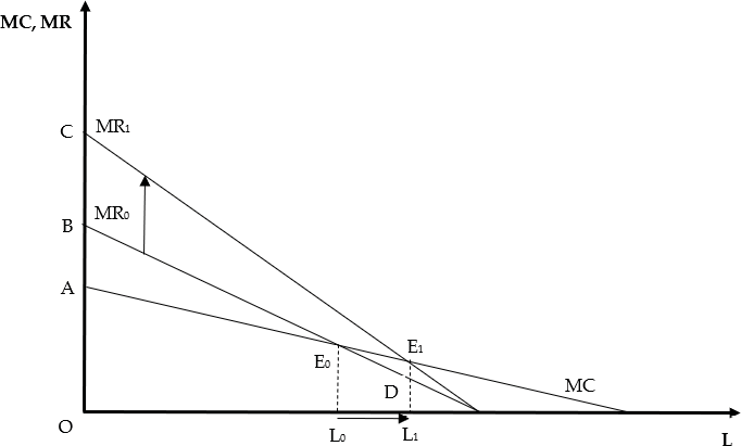
The horizontal axis represents the amount of agricultural land used (in units of area, e.g., hectares). Meanwhile, on the vertical axis, one can read – as the second coordinate of a point located on a given line – the level of MC and MR, expressed in monetary units per unit of agricultural land input, in relation to a homogeneous, unitary plot of land.
MC here means the increase in the cost of production, namely the inputs of production factors other than land (i.e. – in the classical approach – labor and capital), resulting from the increase in land input by one unit. MR is understood here as the increase in TR resulting from the increase in the level of land use by one unit.
MR₀ is the graph of the MR function under conditions where production-linked payments are not applied, thus it includes only revenue from the sale of agricultural produce. MR₁, on the other hand, refers to the situation where production-linked payments are applied. This means that MR₁ includes, in addition to revenues from the sale of agricultural produce, revenues from production-linked payments.
For an agricultural parcel represented by a given point on the horizontal axis of the coordinate system, the ratio of the vertical distance between the line MR0 and the line MR1 to the vertical distance between the horizontal axis of the coordinate system and the line MR0 corresponds to the relation of the amount of support granted to the value of the sale. In other words, this represents the relationship between remuneration sourced from the state and remuneration sourced from the market. Due to the assumption of the independence of the price of the supported agricultural product from the volume of production, this ratio does not change as one moves rightwards along the horizontal axis.
Sadłowski (2017) demonstrated that the application of production-linked payments leads to an increase in production intensity on land already used for agriculture (even in the absence of support) while simultaneously increasing production extensiveness by bringing previously unused land into agricultural production. In the simplified model presented in this study, the effect of a payment-induced increase in inputs (impact on the course of the MC function graph) and revenues from the sale of agricultural produce (impact on the course of the MR function graph) was omitted in relation to land on which production would be carried out even in the absence of support.
The further to the right along the horizontal axis, the less agriculturally useful the land, as the most fertile and accessible plots are used in production first. The graph of the MC function is a downward-sloping line, as the less fertile the land, the lower the amount of labor and capital required to maximize economic outcome (Sadłowski, 2017). This statement concerns the inputs of labor and capital that make up the direct costs of production and not the investment outlays (e.g., the costs of building drainage infrastructure) that make it possible to increase the agricultural suitability of the land. The graph of the MR function is also a downward-sloping line. The negative slope of this line reflects the fact that the most productive land, which generates the highest revenue from the sale of agricultural products, is engaged in production first in the pursuit of maximizing economic outcomes. As less and less fertile and increasingly peripherally located land is involved in the production process (moving to the right along the horizontal axis), the MR from each subsequent unit of land area is lower and lower. The area under the MC curve represents the TC level, while the area under the MR curve represents the TR level.
The effects of changes in factor input prices would be illustrated by a parallel shift of the MC line, while the effects of changes in the price of the supported agricultural product would be illustrated by a parallel shift of the MR line. An increase/decrease in the prices of agricultural inputs or wages would result in an upward/downward shift of the MC line, respectively. Meanwhile, an increase/decrease in the price of the supported agricultural product would be reflected in an upward/downward shift of the MR line.
The optimal level of use of available agricultural land resources when production-linked payments are not applied is determined by the first coordinate of the point where the MC curve intersects the MR₀ curve, i.e., L₀. At this level of land use, the economic outcome, understood as the surplus of TR over TC, is maximized.
However, when agricultural production is subsidized by providing farms with financial support proportional to the volume of production, the factors of production engaged in the production process are remunerated not only by the market (in the form of revenues from the sale of agricultural products) but also by the state (in the form of production-linked payments). This is illustrated by the MR function at position MR₁. In this case, the farm’s equilibrium point will be point E₁, which corresponds to a higher level of land use (L₁ > L₀). Thus, land that was previously (i.e., in the absence of production-linked support) unused for agricultural purposes will now be engaged in production. The length of the segment |L₀L₁| reflects the area of this additional land, i.e., land brought into production as a result of the introduction of production-linked payments. They can be equated with marginal lands (see Csikós and Tóth, 2023); although definitional challenges have not been fully resolved, this concept is relatively frequently used in the literature on the subject.
Therefore, production-linked support acts as an incentive for farms to increase land use, leading to an overall increase in the agricultural land area utilized in the country. However, if resource management is to be rational, there is no justification for expanding this area for reasons other than an improvement in market conditions in agriculture.
4.2 The impact of production support on the remuneration of production factors (distribution sphere)
The remuneration of land, as a resource involved in the production process, is a residual value, representing the surplus of revenues from the sale of agricultural products (in the case of application of production-linked payments, increased by revenues from these payments) over the production costs, which include inputs of production factors other than land. This definition of land remuneration is equivalent to the economic outcome.
Based on Figure 1, it can be noted that in the case without production-linked payments, the total remuneration of land at the farm’s equilibrium point (E₀) is represented by the area of triangle AE₀B. The value of land rent per unit of land area (homogeneous in terms of agricultural suitability) is symbolized by the vertical distance between the MC curve and the MR₀ curve. The value of land rent decreases as we move rightwards along the horizontal axis, corresponding to the inclusion of land with progressively lower agricultural suitability into the production process. The MC curve lies below the MR₀ curve for land with a sufficient level of agricultural suitability to be profitably involved in production, given the production costs and agricultural product prices.
In the case of the use of production-linked payments, land rent consists of two components: one part financed by the market (covered by revenue from the sale of agricultural products) and another part financed by the state (covered by revenue from payments). For a unit of land area (homogeneous in terms of agricultural suitability), the value of the first component is symbolized by the vertical distance between the MC curve and the MR₀ curve, while the value of the second component is represented by the vertical distance between the MR₀ curve and the MR₁ curve. The total remuneration of land at the new equilibrium point (E₁), which, incidentally, corresponds to a greater land input than in the initial situation (L₁ > L₀), is illustrated by the area of the triangle AE₁C. Within this area, the market-financed component is represented by triangle AE₀B and the state-financed component by quadrilateral BE₀E₁C.
To measure the scale of the impact of production-linked payments on the distribution sphere, the following indicators can be used:
– the agricultural subsidization coefficient,
– the coefficient of land rent financing by the state, and
– the payment-to-land rent conversion coefficient.
The presented model allows for a theoretical decomposition of the remuneration of production factors into remuneration from non-land production factors and land rent. For the scenario with production-linked payments, this division can further be separated into the portion financed by the market and the portion financed by the state. The proposed coefficients are structural indicators related to the remuneration of production factors.
4.2.1 Agricultural subsidization coefficient
The agricultural subsidization coefficient is defined as the ratio of the amount of support granted to the total revenue of the farm, which includes revenue from the sale of agricultural products (sourced from the market) and revenue from various state instruments supporting agriculture financially (in the model case under analysis, state support is provided solely in the form of production-linked payments). Therefore, it indicates what portion of the total revenue is derived from state support. In other words, this coefficient shows the percentage of the remuneration of the factors of production involved in agricultural production that is financed by the state.
The agricultural subsidization coefficient (cAAs) is expressed by the formula:
(1)
where:
PRV – the production-linked payment rate (expressed in monetary units per unit of mass of the produced (and sold) agricultural product, e.g., in EUR/t);
V – the volume of supported agricultural products (expressed in units of mass, e.g., in tons);
TR₁ – the total revenue from the production of a given mass of agricultural products, including revenue from the sale of those products and revenue from production-linked payments (expressed in monetary units, e.g., in EUR);
P – the price of the agricultural product (expressed in EUR/t).
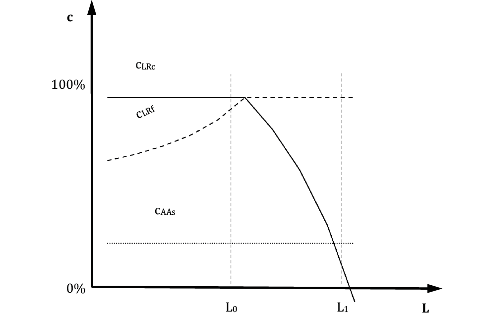
Thus, the agricultural subsidization coefficient is a dimensionless value and can take any value from the closed interval between 0 and 100%. The coefficient equals zero when the remuneration of the factors of production is entirely equivalent to the monetary value of the goods produced, which occurs only when the market is the sole source of financing for inputs. In Figure 1, this situation corresponds to the zero scenario with E₀ as the equilibrium point. However, in conditions where production-linked payments are applied, the value of this coefficient is greater than zero and, under the assumed conditions (the price of the agricultural product and the payment rate being independent of the farm’s production volume), remains constant as one moves to the right along the horizontal axis of the coordinate system, accompanied by a decrease in the agricultural usefulness of the land. The insensitivity of this coefficient to land productivity is illustrated by the graph shown in Figure 2 with a dotted line.
In Figure 1, the value of the agricultural subsidization coefficient for a specific homogeneous unit plot is the ratio of the vertical distance between the MR₀ line and the MR₁ line to the vertical distance between the horizontal axis and the MR₁ line. Meanwhile, the value of this coefficient for a farm at equilibrium point E₁ (i.e., using an amount of land equal to L₁) is the ratio of the area of quadrilateral BDE₁C to the area of trapezoid OL₁E₁C.
4.2.2 Coefficient of land rent financing by the state
Based on Figure 1, it can be stated that production-linked support fully contributes to land remuneration in the case of land that was already being used for agricultural purposes even without this support (up to L₀ inclusive). However, for land that was incorporated into the production process only after the introduction of production-linked payments at rate PRV (to the right of L₀, up to and including L₁), production-linked support partially contributes to land remuneration and partially to the remuneration of other production factors. It can be observed that, as one moves along the horizontal axis of the coordinate system to the right of L₀, an increasingly smaller part of the support linked to production goes towards the remuneration of land, while the importance of this support in creating the remuneration of labor and capital is growing. This means that, as land productivity declines, the market’s share in remunerating labor and capital decreases, while the state’s share increases. In the extreme case of the marginal unit plot L₁, production-linked support fully increases the remuneration of labor and capital while the land rent is zero.
To measure what portion of land remuneration is financed by the state, the concept of the coefficient of land rent financing by the state (cLRf) can be introduced, expressed by the formula:
(2)
where:
PRV – the production-linked payment rate (expressed in monetary units per unit of mass of the produced (and sold) agricultural product, e.g., in EUR/t);
V – the volume of supported agricultural products (expressed in units of mass, e.g., in tons);
TR₁ – the total revenue from the production of a given mass of agricultural products, including revenue from the sale of those products and revenue from production-linked payments (expressed in monetary units, e.g., in EUR);
TC – total cost, i.e., the inputs of production factors other than land in relation to a given area of land (expressed in monetary units, e.g., in EUR).
Like the agricultural subsidization coefficient, the coefficient of land rent financing by the state is a dimensionless value and can take any value from the closed interval between 0 and 100%. Referring to Figure 1, it can be noted that for unit land L₀ and land to the left of it, the state’s share in financing land rent is expressed by the ratio of the vertical distance between the MR₀ line and the MR₁ line to the vertical distance between the MC line and the MR₁ line. This ratio remains constant as one moves to the right along the horizontal axis. For land located to the right of L₀ (up to and including L₁), the state’s share in financing land rent is 100% (since, for this land, both the numerator and the denominator of the fraction expressing this share are the same number corresponding to the vertical distance between the MC line and the MR₁ line), although it does not change the fact that, in absolute terms, land rent decreases as one moves to the right along the horizontal axis of the coordinate system. The graph in the form of a dashed line in Figure 2 illustrates how the value of the coefficient of land rent financing by the state changes depending on the agricultural suitability of the land. For the entire farm at equilibrium point E₁ in Figure 1, the state’s share in financing land rent is expressed by the ratio of the area of quadrilateral BE₀E₁C to the area of triangle AE₁C.
4.2.3 Payment-to-land rent conversion coefficient
The payment-to-land rent conversion coefficient (cLRc) indicates what portion of the financial support provided by the state contributes to the increase in land rent. This indicator can be expressed by the following formula:
(3)
where:
ΔLR – the increase in land rent caused by the introduction of production-linked payments (expressed in monetary units, e.g., in EUR);
PRV – the production-linked payment rate (expressed in monetary units per unit of mass of the produced (and sold) agricultural product, e.g., in EUR/t);
V – the volume of agricultural products supported (expressed in units of mass, e.g., in tons).
Like the indicators expressed in formulas (1) and (2), the payment-to-land rent conversion coefficient is dimensionless, and its possible values range from 0% to 100%. Based on Figure 1, it can be stated that for land used agriculturally even in the absence of production-linked support (up to and including L₀), the value of this coefficient is 100% (both the increase in land rent and the amount of support paid in relation to production generated on a given unit plot are reflected by the vertical distance between the MR₀ line and the MR₁ line, so the quotient of these two values is one). For land that was incorporated into the production process only after the introduction of production-linked payments at rate PRV (to the right of L₀, up to and including L₁), this coefficient is expressed by the ratio of the vertical distance between the MC line and the MR₁ line to the vertical distance between the MR₀ line and the MR₁ line. For land within this range, the coefficient is therefore less than 100% and decreases as one moves right along the horizontal axis of the coordinate system, reaching zero for the marginal unit of land L₁. Observing the graph in the form of a solid line in Figure 2, one can see how this coefficient changes depending on the agricultural suitability of the land. The value of the payment-to-land rent conversion coefficient for all land included in the farm at equilibrium point E₁ in Figure 1 can be calculated as the percentage ratio of the area of quadrilateral BE₀E₁C to the area of quadrilateral BDE₁C.
4.2.4 The phenomenon of “Support Capture” and its measurement
In cases where the land user is not the owner, land rent takes the form of lease rent. A consequence of production-linked payments at least partially converting into land rent is the phenomenon of support being “captured” by landowners through raising lease rent or land sale prices accordingly. In the event of a discrepancy between ownership and use of land, the measure of the degree to which production-linked payments are “captured” by landowners is the payment-to-land rent conversion coefficient (cLRc).
The “capturing” of financial support granted to farmers (land users) by landowners is manifested through increased lease rent rates and higher prices for agricultural land, i.e., the capitalization of payments. This occurs when the landowner is not the same as the land user, and when the land is subject to market transactions. “Capturing” the payments involves incorporating part or all of the support into the lease rent (in the case of leasing) or the land price (in the case of sale), as a consequence of the increased discounted revenues from agricultural land due to the application of financial support instruments for agriculture.
The increase in the stream of discounted revenues from production-linked payments (∆DISVP) can be calculated using the following formula:
(4)
where:
V – the volume of agricultural products supported (expressed in units of mass, e.g., in tons);
cLRc – the payment-to-land rent conversion coefficient (a dimensionless quantity);
PRV – the production-linked payment rate (expressed in monetary units per unit of mass of the produced (and sold) agricultural product, e.g., in EUR/t);
r – the annual interest rate;
(n+1) – the number of years of payment application.
The increase in lease rent for a given year as a result of the introduction of production-linked payments corresponds to the increase in the annual revenue stream caused by the introduction of these payments, whereas the entire increase in the future stream of discounted revenue is capitalized in the land price. Therefore, the first term on the right-hand side of equation (4) represents the theoretical increase in lease rent during the first year of payment application, while the entire sum represents the theoretical increase in land price, assuming the land was sold at the moment the payments were introduced.
The scale and intensity of the “capture” of production-linked payments by landowners depend not only on the predicted future revenue stream from this form of financial support by the potential parties to the agreement (lease or sale). Various institutional factors also play a significant role in this context. In particular, the long-term nature of lease agreements and their inflexibility result in inertia in lease rent rates (Góral and Kulawik, 2015), and legal restrictions on the sale of agricultural real estate may slow down the process of payment capitalization into land prices (Sadłowski, 2017).
This study aligns with the theoretical research on the economic effects of using various financial support instruments in agriculture, which includes among others the works of Chau and De Gorter (2005), Kilian and Salhofer (2008), and Graubner (2018). The issue of use of production-linked payments remains relevant and important, which stems from the need to determine the potential usefulness of this instrument in addressing current agricultural problems – especially as agriculture operates in an increasingly turbulent environment (Despoudi et al., 2020; Budzyńska and Kowalczyk, 2024). This requires recognizing and quantifying the economic effects of using production support, as well as identifying the conditions for its effectiveness and efficiency in achieving the set objectives. The economic effects of using production-linked payments relate to both the production sphere (influence on the level of engagement and directions of use of production factors in agriculture, the volume and structure of agricultural production, and relative prices of agricultural products) and the distribution sphere (influence on the amount and structure of remuneration for production factors).
The added value of this study is manifested in three dimensions: cognitive, practical, and methodological. The recognition of the mechanism by which production-linked payments stimulate the input of production factors in agriculture and the mechanism by which subsidies granted in the form of production-linked payments are transformed into the remuneration of production factors has cognitive value. The model for transforming production-linked payments into the remuneration of production factors can serve as a starting point for econometric research aimed at predicting the economic effects of regulations introduced under agricultural policy (ex-ante evaluation) and measuring the effectiveness and efficiency of agricultural policy instruments (ongoing or ex-post evaluation). The knowledge obtained from such research facilitates the design of agricultural policy tools and the adaptation of instruments to changing socio-economic conditions or revised political objectives. The study also contributes to the development of terminology concerning the economic aspects of direct payments, which promotes the development of methodology and, consequently, the acquisition of more precise and reliable knowledge.
The limitations of the research result in particular from its theoretical nature, scope and adopted assumptions. The credibility of the formulated statements results from their methodical derivation while demonstrating logical connections of consequences as part of the ongoing reasoning. However, the conclusions resulting from the model were not included in the form of hypotheses in order to be tested using statistical methods and empirical data. The study was limited to the analysis of the effects of financial incentives, while the motivations for production decisions of farms may be more complex. Assumptions about price formation and market structures may preclude the extrapolation of results to agricultural systems with significantly different market realities.
The key conclusions from the theoretical research conducted are as follows:
1. As a result of the application of the direct support system, production factors involved in agriculture generate remuneration exceeding the cash equivalent of agricultural products produced by farms.
2. Production-linked payments encourage both more intensive land use and the cultivation of less fertile or more peripherally located land.
3. The agricultural subsidization coefficient measures the relative level of support, remaining constant when payment rate and agricultural product price are independent of production volume.
4. The state’s role in financing land rent grows as land productivity decreases, reaching 100% for marginal land brought into production due to these payments.
5. If payments influence rental rates, landowners “capture” the support, also reflected in land prices; this “capture” is initially limited by rigid rental agreements and legal constraints on land transactions.
6. Unlike area-based support, production-linked payments do not strongly drive rental rate increases but are more susceptible to “capture” by buyers in the supply chain.
Although production-linked payments are not currently used in the CAP, the presented model remains valuable for policymaking in the EU, as CAP revisions or trade agreement renegotiations remain possible. It enables comparisons with other support tools, helping assess their effectiveness under different conditions. Given the increasing instability in agriculture due to economic crises, wars, and rising imports (e.g., from Mercosur), the model can help predict the effects of reintroducing production-linked payments or using them as a temporary stabilization tool. It offers insights into their impact on agricultural markets and farmers’ incomes. The issues addressed in the article can serve as inspiration for further multi-faceted research.
Anania, G., and Pupo D’Andrea, M.R. (2015). The 2013 Reform of the Common Agricultural Policy. Swinnen J. (eds). The Political Economy of the 2014–2020 Common Agricultural Policy: An Imperfect Storm. Brussels. Centre for European Policy Studies.
Baldoni, E., and Ciaian, P. (2023). The capitalization of CAP subsidies into land prices in the EU. Land Use Policy, 134: 1–29. https://doi.org/10.1016/j.landusepol.2023.106900
Bartkowiak, R. (2008). Historia myśli ekonomicznej [History of Economic Thought]. Warszawa. Polskie Wydawnictwo Ekonomiczne.
Beard, N., and Swinbank, A. (2001). Decoupled payments to facilitate CAP reform. Food Policy, 26(2): 121–145. https://doi.org/10.1016/S0306-9192(00)00041-5
Beluhova-Uzunova, R., Mann, S., Prisacariu, M., and Sadłowski, A. (2024). Compensating for the Indirect Effects of the Russian Invasion of Ukraine – Varied approaches from Bulgaria, Poland, and Romania. EuroChoices, 23(1): 11–18. https://doi.org/10.1111/1746-692X.12422
Blaug, M. (1992). The methodology of economics: Or, how economists explain. Cambridge University Press.
Budzyńska, A., and Kowalczyk, S. (2024). Rynki rolne w warunkach wojny [Agricultural markets in war conditions]. Kwartalnik Nauk o Przedsiębiorstwie, 73(3): 5–22. https://doi.org/10.33119/KNoP.2024.73.3.1
Chau, N.H., and De Gorter, H. (2005). Disentangling the Consequences of Direct Payment Schemes in Agriculture on Fixed Costs, Exit Decisions, and Output. American Journal of Agricultural Economics, 87(5): 1174–1181. https://doi.org/10.1111/j.1467-8276.2005.00804.x
Ciaian, P., Baldoni, E., Kancs, d’A., and Drabik, D. (2021). The Capitalization of Agricultural Subsidies into Land Prices. Annual Review of Resource Economics, 13: 17–38. https://doi.org/10.1146/annurev-resource-102020-100625
Council of the European Union (2009). Council Regulation (EC) No 73/2009 of 19 January 2009 establishing common rules for direct support schemes for farmers under the common agricultural policy and establishing certain support schemes for farmers, amending Regulations (EC) No 1290/2005, (EC) No 247/2006, (EC) No 378/2007 and repealing Regulation (EC) No 1782/2003 (OJ L 30, 31.1.2009, p. 16–99). Available at: http://data.europa.eu/eli/reg/2009/73/oj (Accessed on 5 October 2024).
Csikós, N., and Tóth, G. (2023). Concepts of agricultural marginal lands and their utilisation: A review. Agricultural Systems, 204: 103560. https://doi.org/10.1016/j.agsy.2022.103560
Despoudi, S., Papaioannou, G., and Dani, S. (2020). Producers responding to environmental turbulence in the Greek agricultural supply chain: does buyer type matter? Production Planning & Control, 32(14): 1223–1236. https://doi.org/10.1080/09537287.2020.1796138
Donald, P.F., Pisano, G., Rayment, M.D., and Pain, D.J. (2002). The Common Agricultural Policy, EU enlargement and the conservation of Europe’s farmland birds. Agriculture, Ecosystems & Environment, 89(3): 167–182. https://doi.org/10.1016/S0167-8809(01)00244-4
Frascarelli, A. (2020). Direct Payments between Income Support and Public Goods. Italian Review of Agricultural Economics, 75(3): 25–32. https://doi.org/10.13128/rea-12706
Friedman, M. (1953). The Methodology of Positive Economics. Friedman M. Essays in Positive Economics. Chicago. University of Chicago Press.
Góral, J., and Kulawik, J. (2015). Problem of capitalisation of subsidies in agriculture. Problems of Agricultural Economics, 342(1): 3–23. https://doi.org/10.5604/00441600.1147600
Graubner, M. (2018). Lost in space? The effect of direct payments on land rental prices. European Review of Agricultural Economics, 45(2): 143–171. https://doi.org/10.1093/erae/jbx027
Hamulczuk, M., Cherevyk, D., Makarchuk, O., Kuts, T., and Voliak, L. (2023). Integration of Ukrainian Grain Markets with Foreign Markets During Russia’s Invasion of Ukraine. Problems of Agricultural Economics, 377(4): 1–25. https://doi.org/10.30858/zer/177396
Hardt, Ł. (2012). Problem realistyczności założeń w teorii ekonomii [The problem of realisticness of assumptions in economic theory]. Ekonomista, 1: 21–40. Available at: https://ekonomista.pte.pl/Problem-realistycznosci-zalozen-w-teorii-ekonomii,155747,0,2.html (Accessed on 19 December 2024).
Henderson, B., and Lankoski, J. (2019). Evaluating the environmental impact of agricultural policies. OECD Food, Agriculture, and Fisheries Papers, 130. OECD Publishing, Paris. https://doi.org/10.1787/add0f27c-en
Howley, P., Hanrahan, K., and Donnellan, T. (2009). The 2003 CAP reform: Do decoupled payments affect agricultural production? RERC Working Paper Series PUT 09-WP-RE-01. Available at: https://t-stor.teagasc.ie/handle/11019/704 (Accessed on 2 January 2025).
Hristov, J., Clough, Y., Sahlin, U., Smith, H.G., Stjernman, M., Olsson, O., Sahrbacher, A., and Brady, M.V. (2020). Impacts of the EU’s Common Agricultural Policy “Greening” Reform on Agricultural Development, Biodiversity, and Ecosystem Services. Applied Economic Perspectives and Policy, 42(4): 716–738. https://doi.org/10.1002/aepp.13037
Kilian, S., and Salhofer, K. (2008). Single payments of the CAP: where do the rents go? Agricultural Economics Review, 9(2): 96–106. https://doi.org/10.22004/ag.econ.178238
Lankoski, J., and Thiem, A. (2020). Linkages between agricultural policies, productivity and environmental sustainability. Ecological Economics, 178. https://doi.org/10.1016/j.ecolecon.2020.106809
Latruffe, L., and Le Mouël, C. (2009). Capitalization of government support in agricultural land prices: What do we know? Journal of Economic Surveys: 23(4), 659–691. https://doi.org/10.1111/j.1467-6419.2009.00575.x
Matthews, A. (2018). The EU’s Common Agricultural Policy Post 2020: Directions of Change and Potential Trade and Market Effects. Geneva. International Centre for Trade and Sustainable Development.
Mulyk, T., and Mulyk, Y. (2022). Exports of Ukrainian agricultural products to the European Union: analytical assessment, problems and prospects. Three Seas Economic Journal, 3(3): 49–57. https://doi.org/10.30525/2661-5150/2022-3-8
Nedumpara, J.J., Janardhan, S., and Bhattacharya, A. (2022). Agriculture Subsidies: Unravelling the Linkages between the Amber Box and the Blue Box Support. World Trade Review, 21(2): 207–223. https://doi.org/10.1017/S1474745621000288
Niezgoda, D. (2009). Zróżnicowanie dochodu w gospodarstwach rolnych oraz jego przyczyny [Income differentiation in agricultural holdings and reasons for such differentiation]. Zagadnienia Ekonomiki Rolnej, 1: 24–37. Available at: http://www.zer.waw.pl/zroznicowanie-dochodu-w-gospodarstwach-rolnych-oraz-jego-przyczyny,83350,0,2.html (Accessed on 5 October 2024).
OECD (2020). Agricultural Policy Monitoring and Evaluation 2020. OECD Publishing, Paris. https://doi.org/10.1787/928181a8-en
Oleszko-Kurzyna, B. (2007). Postawy rolników wobec grup producentów rolnych [Farmers’ Attitudes Towards Agricultural Producer Groups]. Annales Universitatis Mariae Curie-Skłodowska. Sectio H. Oeconomia, 41(11): 161–176. Available at: https://bc.umcs.pl/Content/20987/PDF/czas9547_41_2007_11.pdf (Accessed on 2 January 2025).
Pilvere I., Nipers A., and Pilvere A. (2022). Evaluation of the European Green Deal Policy in the Context of Agricultural Support Payments in Latvia. Agriculture, 12(12): 2028. https://doi.org/10.3390/agriculture12122028
Pirzio-Biroli, C. (2008). An Inside Perspective on the Political Economy of the Fischler Reforms. Swinnen, J. (eds). The Perfect Storm: The Political Economy of the Fischler Reforms of the Common Agricultural Policy. Brussels. Centre for European Policy Studies.
Potori, N., Kovács, M., and Vásáry, V. (2013). The Common Agricultural Policy 2014-2020: an impact assessment of the new system of direct payments in Hungary. Studies in Agricultural Economics, 115(3): 118–123. https://doi.org/10.7896/j.1318
Ricardo, D. (1996). Principles of political economy and taxation. Amherst. Prometheus.
Sadłowski, A. (2017). Impact of direct payments on the distribution area – model approach. Problems of Agricultural Economics, 350(1): 75–100. https://doi.org/10.30858/zer/83000
Sadłowski, A. (2018a). Coupled support under the first pillar of the Common Agricultural Policy – scope of the member states’ decisiveness and manner of implementation at national level. Roczniki Ekonomiczne Kujawsko-Pomorskiej Szkoły Wyższej w Bydgoszczy, 11: 359–372. Available at: https://cejsh.icm.edu.pl/cejsh/element/bwmeta1.element.ceon.element-a29f7d0b-a918-3f0a-9c2a-41f85e3898c3 (Accessed on 5 October 2024).
Sadłowski, A. (2018b). Jednolita płatność obszarowa – zakres decyzyjności państw członkowskich Unii Europejskiej i sposób wdrożenia w Polsce [The single area payment scheme – the range of decisions made by the member-states of the European Union and the method of its implementation in Poland]. Zagadnienia Doradztwa Rolniczego, 91(1): 5–15.
Sadłowski, A. (2019). The planned reform of the Common Agricultural Policy and its effect on the direct support scheme in Poland. Problems of Agricultural Economics, 360(3): 107–126. https://doi.org/10.30858/zer/112133
Stiglitz, J.E. (2018). Where modern macroeconomics went wrong. Oxford Review of Economic Policy, 34(1–2): 70–106. https://doi.org/10.1093/oxrep/grx057
Swinnen, J. (2010). The Political Economy of the Most Radical Reform of the Common Agricultural Policy. German Journal of Agricultural Economics, 59(1): 37–48. https://doi.org/10.52825/gjae.v59i1.1803
Tangermann, S. (2011). Direct Payments in the CAP post 2013. European Parliamentary Research Service. Belgium. Available at: https://coilink.org/20.500.12592/jmn1cs (Accessed 28 December 2024).