Received: October 31, 2024; Accepted: March 18, 2025; Published: September 30, 2025
Expenditure allocation for Rural Development interventions: main trends and patterns in the choices of the Italian Regions under the CAP 2023-2027
Department of Land, Environment, Agriculture and Forestry, Università di Padova, Italy
*Corresponding author. Email: francesco.pagliacci@unipd.it
Abstract. The introduction of the new delivery model in the 2023-2027 Common Agricultural Policy increased the decision-making and management autonomy of Member States and their regions when implementing Rural Development policies. Thus, understanding the drivers behind allocation choices for rural development funds is crucial. This study analyses the allocation of rural development funds across Italian regions, considering ex-ante share allocation for different types of Rural Development interventions. A cluster analysis is then performed. Different groups of Italian regions are characterised using the indicators developed within the common monitoring and evaluation framework, the allocation of spending in the previous programming period, and other variables. Four clusters of Italian regions are identified: cluster 1 includes rural regions with low urbanisation, prioritising supporting interventions in disadvantaged areas and “environmental” ones; cluster 2 shows large allocation for cooperation interventions; cluster 3 includes regions funding primarily agricultural investments; cluster 4 shows no distinct or unique characteristics. This study is the first one addressing expenditure allocation of the 2023-2027 Common Agricultural Policy. It confirms that expenditure patterns partially couple with geographical and historical similarities, although two main spending priorities (i.e. “environment” and “investments”) persist.
Keywords: EU Rural Development Policy, political economy, cluster analysis, allocation.
JEL codes: D72, O13, Q18.
Index
2.2 Literature review: ex-ante and ex-post expenditure determinants for RD
3.2.1 Input Variables for cluster analysis
3.2.2 Other variables: CMEF and RD expenditure in the previous programming period
Agriculture has been primarily affected by policy interventions, also in the European Union (EU), where the Common Agricultural Policy (CAP) has represented the cornerstone of the European construction, since the origin of the EU (Groupe de Bruges, 1996; Fusco, 2021). CAP objectives have profoundly changed over time to adapt to the transformations of the agricultural sector and the whole society (De Castro et al., 2020). Today, more than in the past, the main objectives of the CAP are mitigating climate change, protecting the environment, landscape and biodiversity, improving the quality and safety of food, social cohesion, and the socioeconomic development of rural areas (Bourget, 2021; European Commission, 2023).
For decades, the CAP has been the most significant EU policy, in terms of budget allocation (De Filippis and Henke, 2010; Matthews, 2017), although its share of the EU budget has halved, from 66% in 1980 to 35% in 2020 (DG Agriculture and Rural Development, 2023). In the current programming period (2023-2027), Italy is the third-largest beneficiary, after France and Spain, of the resources allocated to the CAP from the EU budget (Reg. 2116/2021), receiving 10.5% of the total CAP funds (about 28 billion euros). Just for the Rural Development (RD) Policy, a substantial portion of national funding is added, bringing the total funds for Italy to nearly 37 billion euros. Of this total amount, 48% is allocated to direct payments, while 43% is designated for RD policy (European Commission, 2022).
In the EU, RD Policy has been traditionally managed in a decentralised manner, granting regional autonomy in decision-making and implementations (Dwyer et al., 2007). In Italy, NUTS-2 (Nomenclature des unités territoriales statistiques) regions oversee its management, a role reinforced by the new delivery model. It requires Member States (MS) to develop a National Strategic Plan integrating both direct payments and RD Policy (Langlais, 2023). This shift has extended decentralisation to direct payments as well, now aligning under a need-based assessment, obtained through an in-depth regional-level analysis (Barral, 2023). RD interventions are classified into eight groups, and in Italy, 76 interventions have been selected, letting NUTS-2 regions choose implementation and fund allocation.
In this evolving governance framework, it is important to understand how funding decisions are made, in order to evaluate the effectiveness and equity of CAP distribution, helping to inform future policies that promote rural development and sustainability.
This paper investigates territorial differences in allocation of the RD funds, by analysing decision-making processes in Italy within the 2023-2027 CAP programming period. The primary objective is to understand resource allocation patterns and the key determinants of spending across the Italian regions, offering innovative and updated empirical insights compared to previous studies. While regional differences in total allocation may naturally vary due to their different sizes, it is hypothesised that the percentage distribution of funds across interventions types also differs based on regional characteristics and needs. Additionally, regional governments’ development objectives and policy priorities may shape these allocation choices (Pagliacci and Zavalloni, 2024).
Stemming from this primary objective, this study also seeks to: i) identify clusters of Italian regions that allocate RD funds in a similar way; ii) examine the main drivers behind these allocation patterns, considering socioeconomic, sectoral and geographical factors.
This research contributes to the literature by explaining how decentralised governance and regional policymaking affect fund distribution, offering valuable policy recommendations for both decision-makers and farmers. Given the new governance model, these insights can enhance the efficacy and fairness of future RD policy.
The rest of the paper is structured as follows. Section 2 shows the theoretical background of this work as well as the characteristics of Italian RD Policy in the 2023-2027 programming period. Section 3 presents the datasets used and the main methods adopted. Section 4 reports the results of the analysis, while Section 5 discusses them. Section 6 concludes by highlighting possible implications and formulating hypotheses for future research.
The 2023-2027 CAP was definitively approved in 2021. In the same year, the strategic context regulations of the current CAP (namely, the European Green Deal with its “European climate law” and the “Fit for 55” strategy, as well as the “Farm to Fork” strategy) were also approved.
The Green Deal’s main objective is achieving climate neutrality by 2050 in all EU economic sectors, according to the Paris Climate Agreement (UNFCCC, 2015). In addition, it supports the transformation of the EU into a sustainable, fair and prosperous society with a modern and competitive economy, adopting a holistic and cross-sectoral perspective (Zezza, 2023). The package includes initiatives on climate, environment, energy, transport, industry, agriculture, education and research, sustainable finance, etc., all sectors deeply connected.
Among the Green Deal commitments with the greatest impact on agricultural policy, there are those relating to the “From farm to fork” (European Commission 2020a) and the “EU biodiversity strategy for 2030” (European Commission 2020b). In particular, “From farm to fork” was developed with the specific intention of reducing the environmental and climate footprint of the EU food system, setting some strict environmental targets that EU agriculture must achieve by 2030 (Coderoni, 2023). In doing so, it aims to strengthen EU agriculture’s resilience, ensuring food security, driving the global transition towards competitive sustainability from farm to fork and exploiting new opportunities (Zezza, 2023).
The current 2023-2027 CAP started on the 1st of January 2023. Despite the traditional path dependency that had characterised CAP history (Sotte, 2023), the current programming period represents a clear break from previous ones. The new delivery model is the new governance system that makes the CAP more result-oriented, stressing the role of performance. Precisely in this perspective, increasing freedom of choice is left to local authorities (i.e. national governments, and regional governments), in accordance with the principle of vertical subsidiarity (Bolli et al., 2021).
The new governance model is implemented through National Strategic Plans, developed by each MS after identification of their specific needs. National Strategic Plans outline intervention strategies to achieve EU objectives according to the specific needs of each territory, selecting interventions from a comprehensive range proposed by the Commission, with specific targets and financial plans and after a negotiation phase with the Commission itself. This significantly enhances subsidiarity, allowing MSs to determine how to achieve EU objectives through the National Strategic Plans (Carey, 2019; Matthews, 2021).
The paradigm shift has simplified EU activities but has increased management complexity for MS, particularly in a country like Italy, where both the national and regional governments compete on agricultural policies. However, this shift has led to more targeted and tailored interventions.
The European Commission approved the National Strategic Plan for Italy on 2 December 2022. It establishes a uniform national strategy for the agricultural, agri-food and forestry sectors, managing resources and support from the European Agricultural Guarantee Fund and the European Agricultural Fund for Rural Development (EAFRD). The Strategic Plan provides interventions for direct payments, sectoral support and RD interventions, with a total financial allocation available to the agri-food and forestry sector and rural areas of almost 37 billion euros for the five-year period 2023-2027. The entire financial envelope must pursue the objectives of the CAP. The resources allocated to RD policy come from the EAFRD, which is increased by 55% of national co-financing.
For RD Policy, there are 76 interventions, but four of them refer to risk management and are managed at national level (as in the previous programming period). For remaining RD interventions, Italy decided to implement a management strategy that provides for national interventions with regional elements. Therefore, regional governments plan and manage RD interventions, adapting them to their economic, social and territorial specificities. These RD interventions are implemented through the definition of Regional Programming Complements for RD. They neither contrast with the National Strategic Plan nor add further choices, but detail how the general national strategy has declined at regional level, highlighting which interventions the Region will finance, fund allocation for each of them, and specific conditions relating to each intervention.
In Italy, selected RD Policy interventions belong to eight types (Table 1):
A. environmental, climate and other management commitments (Agro-climatic-environmental interventions);
B. natural or other specific territorial constraints;
C. specific territorial disadvantages resulting from certain mandatory requirements;
D. investments, including investments in irrigation;
E. setting up young farmers and new farmers and starting rural businesses;
F. risk management tools;
G. cooperation;
H. exchange of knowledge and dissemination of information.
A smaller amount of the EAFRD financial resources is also allocated to activities related to Technical Assistance.
Despite the large MS autonomy in resource allocation, the European Commission introduced some financial constraints (ring-fencing), i.e. minimum fund allocations that MSs must guarantee for specific types of intervention, in order to pursue the strategic objectives of the Union. The heaviest one refers to agri-environmental measures, which must represent at least 35% of expenditure for RD policy.
Among the eight RD types of intervention, as shown in Table 1, those that have recorded the largest fund allocation are: agro-climatic and environmental ones and investments, respectively accounting for 28.9% and 26.7% of total resources. Moreover, 18% is reserved for risk management measures (Table 1).
| Type of intervention | EAFRD resources allocated (EUR million) | % EAFRD | |||||||||||||||||
|---|---|---|---|---|---|---|---|---|---|---|---|---|---|---|---|---|---|---|---|
| A. Agro-climatic-environmental interventions | 2099.42 | 28.92 | |||||||||||||||||
| B. Natural or other specific territorial constraints | 6664.71 | 9.16 | |||||||||||||||||
| C. Specific territorial disadvantages resulting from certain mandatory requirements | 14.30 | 0.20 | |||||||||||||||||
| D. Investments, including investments in irrigation | 1937.72 | 26.69 | |||||||||||||||||
| E. Setting up young farmers and new farmers and starting rural businesses | 339.97 | 4.68 | |||||||||||||||||
| F. Risk management tools | 1287.86 | 17.74 | |||||||||||||||||
| G. Cooperation | 591.24 | 8.14 | |||||||||||||||||
| H. Exchange of knowledge and dissemination of information | 96.79 | 1.33 | |||||||||||||||||
| I. Technical support | 188.14 | 2.59 | |||||||||||||||||
| Source: authors’ elaboration on National Rural Network data (2022). | |||||||||||||||||||
2.2 Literature review: ex-ante and ex-post expenditure determinants for RD
Previous literature mainly focused on ex-post investigations on the implementation of agricultural policies, aiming at understanding how government interventions have affected the agricultural sector over time (Anderson et al., 2013). However, very little was said about what affects the allocation of funds within agricultural policies during the planning phase (Fredriksson and Svensson, 2003). For example, Fałkowski and Olper (2014) addressed the role of electoral incentives, Bellemare and Carnes (2015) focused on the personal preferences of legislators, Olper et al. (2014) addressed the pressures from interest groups and institutional contexts, while Pelucha et al. (2016), showed that RD Policy in the Czech Republic was not implemented in accordance with the socioeconomic goals of territorial cohesion.
Referring to ex-post fund allocation, Shucksmith et al. (2005) for the first time tried to assess the impact of the Rural Development Policy at territorial (i.e. regional) level, asking the question of how far CAP expenditure is compatible with objectives of territorial cohesion across the enlarged EU and consistent with the goals of the EU Spatial Development Perspective.
Later, Camaioni et al. (2016) focused on the CAP resource allocation considering NUTS-3 level regions. According to them, allocation is the joint result of top-down policy decisions and bottom-up ability of territories to attract available funds. Thanks to an ex-post econometric analysis on the 2007-2013 RD expenditure, they identified three major drivers for expenditure allocation, which include a “pure spatial effect” (i.e. the influence of the surrounding space on the allocation of RD expenditure) and a negative rurality effect (i.e. the less rural the region, the greater the intensity of spending).
Bonfiglio et al. (2017) analysed the main territorial models of the effective spatial (ex-post) allocation of CAP expenditures by considering knowledge transfer and innovation (KT&I) measures only into the 2007-2013 CAP RD. They confirm that the economy’s structure plays an important role in such a spatial allocation.
Considering the same 2007-2013 programming period, Uthes et al. (2017) also compared the data of the Common Monitoring and Evaluation Framework (CMEF) and the RD policy expenditure levels at NUTS-2 territorial level across the EU. The authors highlighted four different patterns of expenditure allocation, distinguishing the EU regions into four groups: Competitiveness, Environment, Rural Viability, Equal Spending. They were established considering the percentage distribution of RD expenditure among Axes, as provided for in the 2007-2013 CAP. Among the selected groups, the largest difference was observed between regions in the “Competitiveness group” and those in the “Environment group”, the latter one having a larger share of arable land and less permanent grassland, a smaller physical and economic farm size, greater workforce, less land in less favoured areas, a higher share of extensive arable land and a lower share of extensive grazing. On the contrary, the regions of the “Environment group” also show a higher proportion of UAA within natural areas. Uthes et al. (2017) once again demonstrate the feasibility of identifying expenditure patterns and validate the use of CMEF indicators in explaining them. Most importantly, their findings highlight a strong coherence between spending priorities, regional needs and development prospects.
Zasada et al. (2018) focused on European regions with above-average expenditures for natural capital measures within RD Policy in the 2007-2011 period. They aim to understand the drivers behind such spending priorities related to local socioeconomic and agricultural contexts. The analyses identified six different spending patterns for European regions. The results show that the adoption of natural capital-oriented spending models is only partially influenced by environmental and agricultural factors, with a higher incidence of larger farms and regions with high purchasing power and population density. However, a weak correlation exists between natural capital investments and ecologically significant areas such as Natura 2000 sites or High Nature Value farmland. This shows that these areas don’t receive enough funds. Socioeconomic and agricultural indicators have limited influence, reflecting criticisms about the RD Policy’s lack of attention to local needs (Copus and Dax, 2010; Piorr and Viaggi, 2015).
Lastly, Pagliacci and Zavalloni (2024) investigated the factors that influence the allocation of funds for some specific objectives of the CAP (i.e. environmental objectives), considering the European 2014-2020 RD. Compared to previous articles, which mainly analysed the ex-post determinants, they mostly focused on the determinants behind the decision-making process. Their results suggested that per capita GDP and population density positively correlate with higher environmental support, whereas greater decentralisation of the management of funds (i.e. at regional and not at national level) is negatively correlated with environmental support. Therefore, Pagliacci and Zavalloni (2024) suggested that maintaining central control over the financial allocation could promote greater environmental sustainability in the agricultural sector.
However, to the authors’ best knowledge, no studies have yet addressed the 2023-2027 CAP.
This study applies quantitative analyses to understand the distribution of RD expenditure in Italian regions. Firstly, a cluster analysis is conducted considering 21 NUTS-2 level regions in Italy, i.e. 19 Italian Regioni and 2 Province Autonome1. A hierarchical clustering is applied to a set of input variables that refer to RD expenditure allocation (see section 3.2), and that are preliminarily standardised. For the cluster analysis, Euclidean distance and Ward’s method are used to determine distance between statistical units and clusters (Ward, 1963; Murtagh and Legendre, 2014). In particular, the Ward’s method aims to minimise the variance within each cluster by merging the clusters that minimise the increase in the total sum of squared distances. Despite its strengths, which make it particularly suitable when clusters show different sizes and densities, the Ward’s method might be sensitive to outliers, leading to biased results if there are non-random patterns of missing data or if the underlying assumptions of normality and equal variances are violated (Ward, 1963).
Having selected a hierarchical cluster analysis, the choice of the number of clusters is defined ex post, under the well-known trade-off between the number of clusters considered and their homogeneity. The cluster analysis is conducted using the R software (R Core Team, 2024), and “fpc” package (Hennig, 2024).
After clustering, group description is done by submitting clustering variables to ANOVA (analysis of variance) to find significant differences among the clusters. Subsequently, a Tukey HSD (Honest Significant Differences) test is also conducted to verify which clusters differ significantly from each other (Yandell, 1997). The results of these two tests are used to support cluster labelling.
Then, a further phase of the work aims to verify whether regions belonging to the same cluster also show other similarities at structural level, i.e. considering other descriptive variables, such as: socioeconomic, sector-based (i.e. agriculture) and environmental variables. This analysis is accomplished by performing an ANOVA test for each variable to verify if at least one cluster behaved differently from the others, and then a Tukey HSD test to identify which one(s) differ from each other.
As a final stage of our investigation, and in order to further characterize the identified clusters and explore potential correspondences between planned expenditure and characteristics of the Italian regions, a correlation analysis is conducted. Correlation coefficients are calculated between share of funds allocated to various types of interventions and CAP context indicators (CMEF), but also allocation of public resources during the previous 2014–2022 programming period (see Section 3.2). The choice of CMEF indicators, raw data and territorial subdivision of the analysis (NUTS2) is inspired by Uthes et al. (2017), although they referred to a previous programming period.
Correlation analysis is carried out using Spearman’s method, after verifying that the assumption of linearity is hardly met. All analyses are performed using R (R Core Team, 2024).
3.2.1 Input Variables for cluster analysis
Cluster analysis is grounded on input data that encompass the shares allocated by each region to each type of intervention in the 2023-2027 CAP out of the total RD expenditure. As mentioned above, RD Policy is jointly funded by the EU and the MS. For the analysis, the overall allocation of public resources is considered, according to the 8-group taxonomy already shown in Table 1. As Risk Management Tools are managed at national central level, they are not considered.
In addition to the seven types of intervention, three additional input variables are added: i) share of expenditure allocated to “technical assistance”; ii) total allocation of RD expenditure; iii) number of different activated interventions (as a proxy for heterogeneity of interventions at regional level)2. Table 2 shows summary statistics for input variables.
| NUTS-2 Regions | Clustering variables | ||||||||||||||||||
|---|---|---|---|---|---|---|---|---|---|---|---|---|---|---|---|---|---|---|---|
| A. Agro-climatic-environmental (%) | B. Nature & territorial constraints (%) | C. Specific disadvantages (%) | D. Investments (%) | E. Young farmers (%) | G. Cooperation (%) | H. Knowledge (%) | Technical assistance (%) | Total (EUR million) | Number of interventions | ||||||||||
| ITF1-Abruzzo | 36.30 | 12.79 | 0.29 | 27.92 | 7.56 | 9.26 | 2.33 | 3.55 | 343.90 | 33 | |||||||||
| ITF5-Basilicata | 31.96 | 9.93 | 0.00 | 36.59 | 8.17 | 8.90 | 1.14 | 3.31 | 452.94 | 37 | |||||||||
| ITH20-Bolzano | 39.36 | 35.86 | 0.00 | 11.16 | 6.62 | 6.49 | 0.18 | 0.33 | 271.87 | 18 | |||||||||
| ITF6-Calabria | 42.29 | 3.84 | 0.00 | 35.69 | 5.12 | 8.85 | 0.90 | 3.31 | 781.29 | 39 | |||||||||
| ITF3-Campania | 33.32 | 15.62 | 0.00 | 31.79 | 3.76 | 11.79 | 0.98 | 2.75 | 1149.61 | 35 | |||||||||
| ITH5-Emilia-Romagna | 35.71 | 11.17 | 0.39 | 30.93 | 6.77 | 10.32 | 2.18 | 2.53 | 913.22 | 45 | |||||||||
| ITH4-Friuli-Venezia Giulia | 33.75 | 11.05 | 0.88 | 37.57 | 5.30 | 7.12 | 1.24 | 3.09 | 226.25 | 29 | |||||||||
| ITI4-Lazio | 33.42 | 8.74 | 1.16 | 27.56 | 10.78 | 13.90 | 1.12 | 3.32 | 602.06 | 31 | |||||||||
| ITC3-Liguria | 17.12 | 5.20 | 0.52 | 54.75 | 8.40 | 8.36 | 2.33 | 3.31 | 207.04 | 48 | |||||||||
| ITC4-Lombardy | 17.79 | 11.12 | 0.00 | 49.44 | 4.58 | 10.66 | 3.79 | 2.62 | 764.50 | 39 | |||||||||
| ITI3-Marche | 34.75 | 11.49 | 0.20 | 34.08 | 3.53 | 10.45 | 3.45 | 2.05 | 390.88 | 38 | |||||||||
| ITF2-Molise | 36.27 | 18.63 | 0.00 | 27.14 | 5.07 | 5.00 | 4.32 | 3.57 | 157.71 | 21 | |||||||||
| ITC1-Piedmont | 34.70 | 5.71 | 0.79 | 35.46 | 5.29 | 12.18 | 2.70 | 3.17 | 756.40 | 50 | |||||||||
| ITF4-Puglia | 35.91 | 1.27 | 0.00 | 41.04 | 4.22 | 12.74 | 1.50 | 3.31 | 1184.88 | 41 | |||||||||
| ITG1-Sardinia | 39.88 | 20.26 | 0.00 | 26.24 | 4.88 | 7.64 | 0.49 | 0.62 | 819.49 | 30 | |||||||||
| ITG2-Sicily | 46.54 | 15.78 | 0.00 | 21.56 | 6.81 | 7.09 | 0.52 | 1.70 | 1467.61 | 30 | |||||||||
| ITI1-Tuscany | 37.61 | 7.51 | 0.40 | 33.51 | 6.61 | 11.07 | 2.30 | 0.99 | 748.81 | 54 | |||||||||
| ITH10-Trento | 21.94 | 25.13 | 0.00 | 35.93 | 6.07 | 7.36 | 0.55 | 3.02 | 198.96 | 17 | |||||||||
| ITI2-Umbria | 31.44 | 6.07 | 0.29 | 40.63 | 2.51 | 14.61 | 1.45 | 3.01 | 518.60 | 44 | |||||||||
| ITC2-Valle d’Aosta | 35.42 | 33.64 | 2.18 | 17.69 | 1.09 | 8.43 | 0.63 | 0.92 | 91.85 | 27 | |||||||||
| ITH3-Veneto | 25.09 | 10.91 | 0.85 | 38.95 | 8.56 | 9.93 | 3.58 | 2.13 | 824.56 | 44 | |||||||||
| Source: authors’ elaboration on National Rural Network data (2022). | |||||||||||||||||||
3.2.2 Other variables: CMEF and RD expenditure in the previous programming period
The analysis includes an additional set of variables. The CAP context indicators in the CMEF are developed by the European Commission to evaluate the results of the CAP and examine fund allocation. There are 45 main indicators, each of them with multiple sub-indices. Almost all of them are available at NUTS-2 level, hence being useful for this analysis. Twelve cross-cutting socio-economic indicators allow regions to be framed jointly (e.g., population, population density, employment rate). Moreover, there are eighteen sectoral indicators, specific to the agricultural sector, and fifteen environmental indicators, which are useful to understand environmental conditions of regions, the strategies implemented for its protection as well as the impacts of the agricultural sector on the environment. The selected sources for these indicators are the following: EUROSTAT; Farm Accountancy Data Network (FADN); European Environmental Agency (EEA); CORINE Land Cover (CLC); DG Agriculture and Rural Development; Natura 2000 Barometer Statistics Report and Joint Research Centre (JRC Ispra). The most recent indicators available have been updated in June 2020. For those indicators that show poor updates, data from ISTAT website (https://www.istat.it/) are retrieved and used.
Given that they refer to a period which is previous to the start of the current programming period, they are not affected by spending choices, hence they can be used in this analysis.
Lastly, expenditure allocations in the previous 2014-2022 CAP programming period is also considered, breaking them down by priority of intervention and technical assistance, both in absolute and percentage terms.
This broad set of variables is used to: i) characterise and provide proper labels to the clusters of regions (e.g. in order to verify the presence of similar characteristics for the regions belonging to the same cluster); and ii) assess the existence of correlations between these additional variables and the percentage allocation of funds across RD interventions, in the Italian regions.
Figure 1 displays the results of hierarchical clustering through a dendrogram. Observing its structure, it is possible to highlight, as a best partition option, a four-cluster partition for the Italian NUTS-2 level regions.
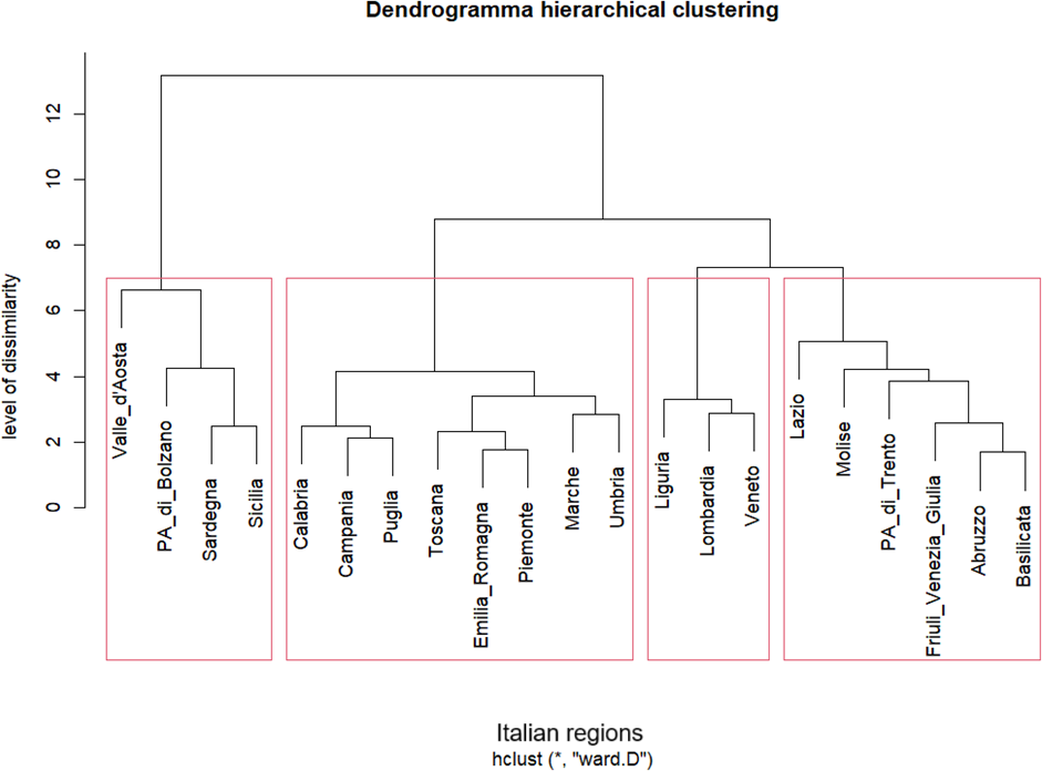
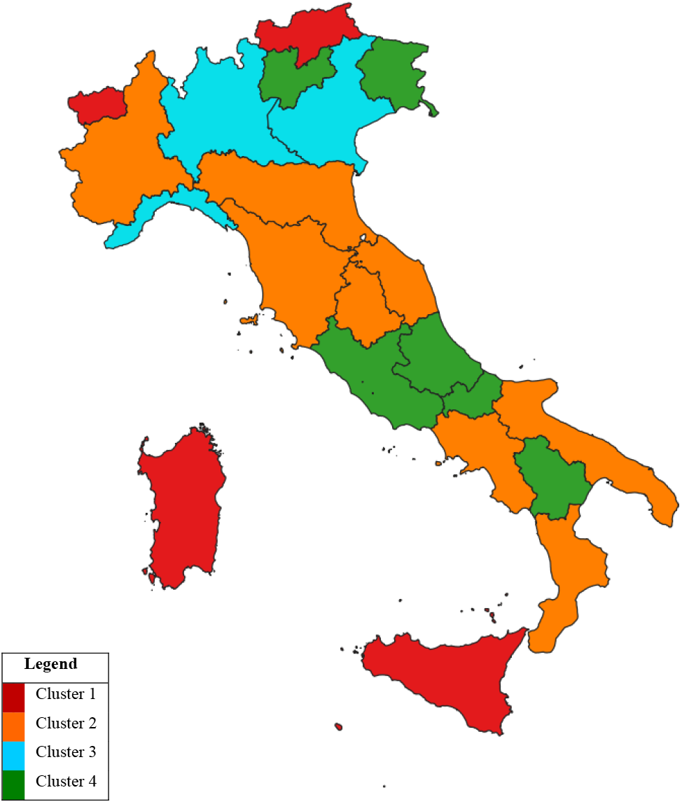
Clusters have different size as well as different average characteristics (Table 3). The smallest group consists of just three regions, while the largest one includes eight regions. Figure 2 maps the clusters in Italy.
| Cluster | Average value (Italy) | ||||
|---|---|---|---|---|---|
| 1 Regions with disadvantages |
2 Cooperation regions |
3 Investment regions |
4 Equal spending regions |
||
| PA di Bolzano Sardegna Sicilia Valle d’Aosta |
Calabria Campania Emilia-Romagna Marche Piemonte Puglia Toscana Umbria |
Liguria Lombardia Veneto |
Abruzzo Basilicata Friuli-Venezia Giulia Lazio Molise PA di Trento |
||
| A. Environment (%) | 40.30 | 35.72 | 20.00 | 32.27 | 32.07 |
| B. Nature & territorial constraints (%) | 26.39 | 7.84 | 9.08 | 14.38 | 14.42 |
| C. Specific disadvantages (%) | 0.55 | 0.26 | 0.46 | 0.39 | 0.41 |
| D. Investments (%) | 19.16 | 35.39 | 47.71 | 32.12 | 33.60 |
| E. Young farmers (%) | 4.85 | 4.73 | 7.18 | 7.16 | 5.98 |
| G. Cooperation (%) | 7.41 | 11.50 | 9.65 | 8.59 | 9.29 |
| H. Knowledge (%) | 0.46 | 1.93 | 3.23 | 1.78 | 1.85 |
| Technical Assistance (%) | 0.89 | 2.64 | 2.69 | 3.31 | 2.38 |
| TOT (EUR million) | 662.7 | 805.46 | 598.70 | 330.3 | 599.29 |
| Number of Interventions | 26.25 | 43.25 | 43.67 | 28.00 | 35.29 |
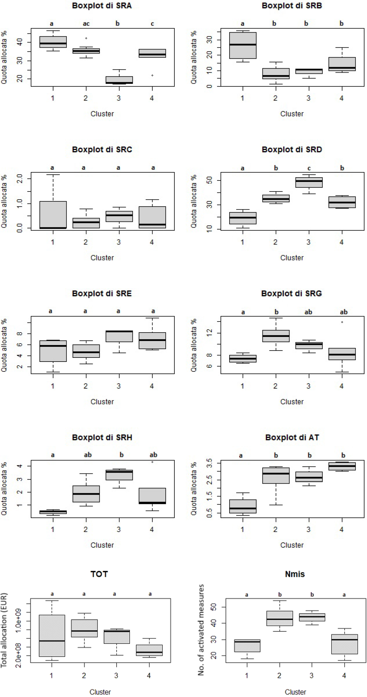
Thanks to the ANOVA and Tukey HSD tests, the clustering input variables are analysed to identify those that contribute most to the identification of each cluster. It is important to note that the limited number of statistical units, in relation to the four clusters, might have reduced the ability to detect statistically significant differences between them. The results of these analyses are reported in Annex A, which displays boxplots for each of the selected input variables.
The results of the ANOVA suggest no significant differences between the four clusters regarding the percentage allocation of “Specific disadvantages” interventions, “Young farmers” interventions and the overall allocation of RD Policy funds. Thus, the analysis of the four clusters is based on the remaining seven variables.
Cluster 1 is labelled as “regions with disadvantages”. It shows a significantly higher-than- average allocation for “Nature & territorial constraint” interventions (support to areas with natural disadvantages or other specific constraints), equal to 26.39%. Cluster 1 also has the highest allocation level in agro-climatic-environmental interventions, equal to 40.30%, and the lowest allocation in investment interventions.
Cluster 2 is named as “cooperation regions”. It has the highest allocation for interventions related to cooperation in agriculture. On the other hand, it shows an average allocation for agro-climatic-environmental interventions, investment-related ones and those for knowledge and information exchange (AKIS). Cluster 2, together with cluster 3, is also the one that activated the largest number of interventions, about 43.
Cluster 3 is labelled as “investment regions”, being characterised by a significantly higher allocation of funds to the interventions for investments. They are almost equal to 50% of the total allocation. The allocation for “exchange of knowledge and information” interventions is also higher than the average (3.23% vs. 1.85%). On the other hand, there is substantially less commitment to agro-climatic-environmental interventions, to which only 20% of resources are dedicated, half of what cluster 1 allocates and about 12% less than the average.
Cluster 4 includes “equal spending” regions, i.e. those regions not showing significant differences compared to the other three clusters. In this cluster, types of intervention show values close to the general average, with deviation usually less than one percentage point. However, it is clear that the regions of this cluster planned “smaller” budgets than the other regions, they allocate the lowest budget and also activate the fewest interventions (this can be deduced from the visual comparison of the medians in the boxplots, Tukey’s HSD test did not show significant differences between the four clusters).
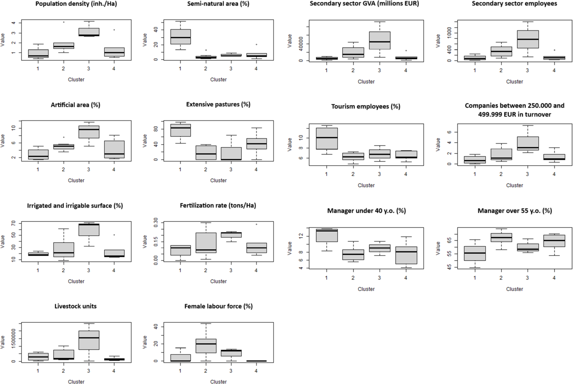
To further expand cluster classification, it is possible to identify the statistically significant differences among clusters and the additional CAP context indicators. Of the large set of variables, 20 of them have proven to be helpful for characterization (see Annex B for some boxplots of the variables that show significant differences between the clusters). In what follows, there is a brief description of each cluster, under these additional covariates.
The regions included in cluster 1 are characterised by an extremely higher endowment of semi-natural areas (31.05% on average, but with a large standard deviation, equal to 13.79%) than the other clusters. Consequently, it is also the group with the lowest share of urbanised areas (only 2.79%, compared to an average of 4.91) (Annex B). This is coherent with low population density (95 inhabitants/km2), significantly lower than the general average (196 inhabitants/km2). Cluster 1 also has a very high share of employment in the tourism sector (9.89% ± 2.28%), which is higher than the Italian average (7.10%). Finally, the regions belonging to cluster 1 appear to be those with the greatest involvement of young farmers in the management of farms. Indeed, 12.19% of companies are led by farmers under 40, while the average value is 8.70%. This is also confirmed by the consequent lower number of farm managers over 55, who represent only 55.49% of the total (but with a large standard deviation, 7,40%).
Cluster 2 does not show specific elements of difference. One item, however, appears worthy of interest: female employment in agriculture. The total and male non-family workforce does not show differences compared to the other clusters. In contrast, for the female workforce the difference is great both in absolute (Annual Work Units – AWUs) and relative terms. In cluster 2, 19.42% of the total workforce are women (although its standard deviation is 13.48%), while the Italian average is just 9.39%.
Cluster 3 has the highest population density: 338 inhabitants/km2 (compared to an average of 196 inhabitants/km2 in Italy). This value is significantly higher than the one observed in clusters 1 and 4 (for this variable, the Tukey HSD output is statistically significant). Cluster 3 is also the group with the most urbanized regions, with 8.81% of its area characterised by urban surface, compared to only 6.21% of the area covered by semi-natural areas, below the average of around 10.37%. The presence of manufacturing companies is therefore large, and this is confirmed by the number of employees in the secondary sector, twice as high as the Italian average, and by all the other economic indices. The agricultural sector follows a similar trend. Cluster 3 shows the largest share for irrigated/irrigable area (56.70% of the total, but with standard deviation of 17.52%), amount of fertilisers distributed and also livestock units. All these are indicators of the high level of specialisation and productivity of farms in these regions. In this way, the percentage of farms of large economic size is significant. Companies between 250,000 and 499,999 EUR in turnover represent 4.17% of the total, the Italian average does not reach 1.80%.
For cluster 4, as observed in the cluster labelling phase, no distinctive features emerge compared to the general average of the Italian regions. The average population density is 142 inhabitants/km2, the regional territory is covered by 7.29% of semi-natural areas (but with large standard deviation, equal to 6.23%) and 4.02% of artificial areas. 5.24% of the population is employed in the primary sector, 22.08% in the secondary sector and 72.68% in the tertiary sector.
As a conclusive test, the analysis of correlation coefficients suggests that demographic variables, economic variables, characteristics of the agricultural sector, and the allocation of funds in the past programming period correlate with current RD expenditure allocation.
On the contrary, total expenditure is positively correlated with total population and population density, as expected. Moreover, more populous regions allocate more funds to investments but less funds to address natural constraints. At the same time, there is a negative correlation between “Natural or other specific territorial constraints” interventions and urbanisation rate. Conversely, larger shares for semi-natural or protected areas couple with larger shares of funds, for interventions for Natural or other specific territorial constraints.
Referring to the economic variables, there is a positive correlation between per capita GDP and the total allocations of funds. Total labour productivity is negatively associated with Agro-climatic-environmental interventions, while it is positively correlated with the funds for natural disadvantages. Regions with larger farms allocate more funds for investment but less for environmental interventions. A more detailed overview of the correlation analysis is reported in Table 4.
| Descriptive variables | Unit | RD interventions 2023-2027 | |||||||||||||||||
|---|---|---|---|---|---|---|---|---|---|---|---|---|---|---|---|---|---|---|---|
| A. Agro-climatic-environmental (%) | B. Nature & territorial constraints (%) | C. Specific disadvantages (%) | D. Investments (%) | E. Young farmers (%) | G. Cooperation (%) | H. Knowledge (%) | Technical Assistance | TOT | Number of Interventions | ||||||||||
| Demographic variables | Regional surface | ha | - | - | - | - | - | 0.387 (0.084) | - | - | 0.847 (0.000) | 0.456 (0.038) | |||||||
| Total population | 1000 inhab. | - | -0.371 (0.098) | - | - | - | 0.526 (0.016) | - | - | 0.804 (0.000) | 0.486 (0.026) | ||||||||
| Population density | Inhab/km2 | - | -0.443 (0.046) | - | 0.408 (0.068) | - | 0.494 (0.024) | 0.385 (0.085) | - | 0.547 (0.011) | 0.499 (0.021) | ||||||||
| Urban area | % total | - | -0.454 (0.039) | - | - | - | - | - | - | 0.482 (0.027) | 0.439 (0.047) | ||||||||
| Population Urban area | % total | - | -0.482 (0.027) | - | - | - | 0.408 (0.067) | - | - | 0.457 (0.037) | 0.426 (0.054) | ||||||||
| Regional protected area | % total | - | 0.443 (0.044) | 0.425 (0.055) | -0.382 (0.087) | - | - | - | -0.402 (0.07) | -0.397 (0.075) | |||||||||
| Economic variables | GDP per capita | EUR/inhab | - | -0.386 (0.085) | - | - | - | 0.519 (0.017) | - | - | 0.651 (0.002) | 0.563 (0.008) | |||||||
| Primary sector GVA | % total | 0.568 (0.008) | - | -0.729 (0) | - | - | -0.404 (0.071) | - | - | - | - | ||||||||
| Secondary sector GVA | % total | -0.416 (0.062) | - | - | - | - | 0.561 (0.008) | - | - | - | |||||||||
| Total employment | 1000 persons | - | -0.416 (0.062) | - | - | - | 0.558 (0.01) | - | 0.691 (0.001) | 0.59 (0.005) | |||||||||
| Employed in primary sector | 1000 persons | - | - | - | - | - | 0.449 (0.042) | - | 0.936 (0) | 0.382 (0.087) | |||||||||
| Employees in the secondary sector | 1000 persons | - | -0.391 (0.081) | - | - | - | 0.596 (0.005) | 0.45 (0.041) | - | 0.645 (0.002) | 0.622 (0.003) | ||||||||
| Employed in tourism | % total | - | 0.449 (0.042) | - | - | - | - | -0.531 (0.013) | -0.47 (0.032) | - | - | ||||||||
| Unemployment rate 15- 74 years old | % total | - | 0.374 (0.096) | - | - | - | - | - | - | 0.391 (0.08) | 0.388 (0.083) | ||||||||
| Annual working unit | AWU | - | - | - | - | - | 0.427 (0.055) | - | - | 0.947 (0.000) | 0.39 (0.081) | ||||||||
| Total Labour Productivity | EUR/person | -0.422 (0.058) | - | 0.433 (0.05) | - | - | - | - | - | -0.447 (0.044) | - | ||||||||
| Labour Productivity in Primary sector | - | -0.381 (0.09) | - | - | - | - | - | - | - | - | - | ||||||||
| Labour Productivity in Secondary sector | - | -0.488 (0.026) | - | - | - | - | - | - | - | -0.438 (0.049) | - | ||||||||
| Large companies (EUR 250,000-499,000) | % of total | -0.423 (0.057) | -0.374 (0.096) | 0.397 (0.074) | 0.448 (0.043) | - | - | 0.421 (0.057) | - | - | 0.571 (0.007) | ||||||||
| Sectoral variables | Agricultural holding | N. | - | -0.399 (0.074) | - | - | - | 0.427 (0.055) | - | - | 0.918 (0.000) | 0.382 (0.087) | |||||||
| SAT | ha | - | - | - | - | - | 0.37 (0.099) | - | - | 0.890 (0.000) | 0.393 (0.078) | ||||||||
| UAA | ha | - | - | - | - | - | 0.408 (0.068) | - | - | 0.912 (0.000) | 0.389 (0.081) | ||||||||
| Organic area | % total UAA | 0.486 (0.027) | - | - | - | - | - | - | - | 0.486 (0.027) | - | ||||||||
| Irrigated and irrigable areas | % total UAA | -0.371 (0.098) | - | - | - | - | - | - | - | - | - | ||||||||
| Arable land | % of total UAA | - | - | - | 0.403 (0.071) | - | 0.451 (0.042) | 0.676 (0.001) | - | - | 0.514 (0.017) | ||||||||
| Permanent grassland and meadow | % of total UAA | - | 0.439 (0.048) | - | -0.41 (0.066) | - | -0.486 (0.027) | -0.529 (0.014) | - | -0.566 (0.008) | -0.597 (0.004) | ||||||||
| Permanent crops | % of total UAA | - | -0.487 (0.027) | - | - | - | - | - | 0.433 (0.05) | - | - | ||||||||
| Companies with a young and graduate leader | % total | - | -0.47 (0.031) | - | 0.387 (0.083) | 0.452 (0.04) | 0.511 (0.018) | - | - | 0.517 (0.016) | |||||||||
| Past funds | Priority 1 - Fostering knowledge transfer and innovation in agriculture, forestry and rural areas | - | - | - | - | - | - | - | - | - | - | - | |||||||
| Priority 2 - Enhancing the viability and competitiveness of all types of agriculture, and promoting innovative farm technologies and sustainable forest | - | -0.409 (0.067) | - | - | 0.606 (0.004) | - | - | 0.416 (0.06) | - | - | - | ||||||||
| Priority 3 - Promoting food chain organisation, including processing and marketing of agricultural products, animal welfare and risk management in agriculture | - | - | - | - | - | - | 0.499 (0.023) | - | - | 0.431 (0.052) | 0.38 (0.089) | ||||||||
| Priority 4 - Restoring, preserving and enhancing ecosystems related to agriculture and forestry | - | 0.522 (0.016) | 0.564 (0.009) | - | -0.644 (0.002) | - | -0.526 (0.016) | -0.557 (0.009) | - | - | -0.524 (0.015) | ||||||||
| Priority 5 - Promoting resource efficiency and supporting the shift towards a low carbon and climate resilient economy in agriculture, food and forestry sectors | - | - | -0.487 (0.027) | - | 0.506 (0.02) | - | - | - | - | - | 0.402 (0.071) | ||||||||
| Priority 6 - Promoting social inclusion, poverty reduction and economic development in rural areas | - | -0.408 (0.068) | - | - | - | - | - | 0.461 (0.035) | 0.436 (0.048) | -0.378 (0.092) | - | ||||||||
| Total public expenditure | - | - | - | - | - | - | 0.425 (0.056) | - | - | 0.983 (0) | 0.391 (0.08) | ||||||||
| Note: Only correlation coefficients, with p-values <10% are reported. Source: our elaboration on ISTAT (http://dati.istat.it/) and EU Commission data (https://agridata.ec.europa.eu/extensions/DataPortal/cmef_indicators.html). | |||||||||||||||||||
Lastly, the distribution of funds between the 2014-2022 and 2023-2027 programming periods shows continuity in priorities, with a focus on farm competitiveness and over environmental measures (Table 4).
The analysis of the allocation of RD Policy expenditure in Italy, in the 2023-2027 programming period, seems to confirm the results of previous studies on similar topics. The territorial imbalances produced by the CAP and its – at least partial – inconsistency with the EU’s cohesion and convergence objectives have already been debated (see for example Esposti, 2007; 2011). Moreover, many studies have investigated how little “rural” the allocation of RD Policy spending is, in fact supporting less rural regions compared to what is stated in its political intentions (Camaioni et al., 2013; Shucksmith et al., 2005; Crescenzi et al., 2011). Similarly, such a trend also seems to be confirmed by this study, as shown by the correlation analyses conducted. If it is reasonable to expect a positive correlation between total expenditure allocation and the total amount of people living in each region, or their regional area, since larger regions can correspond RD Policy with higher budget, it is much more complex to justify the existence of a positive correlation between total expenditure and three major indicators of the presence of a larger urban population: population density (inhabitant/km2), population in urban areas (% total) and the share of urban territory (% total). It can be deduced that, also in the 2023-2027 programming period, urban regions, also due to their likely better administrative capacity (Charron et al., 2021), were more successful in attracting RDP funds, thus feeding a counter-selection mechanism that has already been verified in the past.
However, when dealing with the allocation of RD Policy budget across regions, and in order to identify which Italian regions share similar spending behaviours, the results of the hierarchical cluster analysis seem inconsistent from a geographical point of view, with neighbouring regions showing different patterns. Nevertheless, if one looks at the structure of the dendrogram at a deeper level, some geographical coherences can be found. It is possible to identify micro-clusters of regions that spend in a similar way and are also neighbours. For example, the cluster 2 “cooperation regions” can be divided into two further sub-groups of neighbouring regions: on the one hand, Piedmont, Emilia-Romagna, Tuscany, Umbria and Marche; on the other, Puglia, Campania and Calabria. This further segregation of the dendrogram turns into greater similarity in expenditure allocation within the two subgroups. Also, within cluster 1 it is possible to identify a sub-cluster composed of the two Italian islands: Sicily and Sardinia. The same applies to clusters 3 and 4 even if the phenomenon is less clear.
This could eventually suggest the existence of something similar to a “local agglomeration effect” (already identified by Camaioni et al., 2016) even at NUTS 2 level for Italy. According to this, neighbouring regions with high RD Policy support also tend to induce more support in the region in question and vice versa. The phenomenon had been studied at a more detailed level of disaggregation (NUTS 3, compared to NUTS 2 in this study) and over a more extended programming period in past studies, e.g., the one by Camaioni et al. (2016) and by Crescenzi et al. (2011). Nevertheless, it is important to highlight the added value of the current study. Indeed, it confirms similar results, also when considering ex-ante fund allocation and even under the current 2023-2027 programming period. This is true even though the current programming period is characterised by a new governance system, i.e. the new delivery model.
Moreover, when identifying the determinants of the expenditure behind clusters, it is possible to understand the regional structural characteristics that led to those specific allocation choices.
Similar analyses have been conducted in the past, referring to previous programming periods. The clustering made by Uthes et al. (2017) has many similarities with this one, even though more than ten years and two programming periods have passed. They traced all Italian regions into two groups: Veneto, Liguria and Friuli Venezia-Giulia to the “Competitiveness” group while all the others to the “Environment” group. It is interesting to see that Veneto and Liguria were assigned to the group of “Competitiveness” regions, as it is the case in the present study. However, in this study, given the change in name of the interventions in the new programming period, this group has been labelled “Investment Group”. However, the expenditure targets are similar, as demonstrated by the correlation analyses conducted between investment interventions of the 2023-2027 programming period and the allocation for Priority 2 – Competitiveness and profitability of farms – of the 2014-2020 CAP.
Also, the characterization made by Uthes et al. (2017) about the “Competitiveness” and the “Environment” groups shows clear similarities with our description respectively of “Investment” group and “Disadvantaged” regions.
The identification of similarities, based on spending behaviour in the 2007-2013 and 2023-2027 programming periods, as well as the clear correlation between the expenditure allocation for related objectives between the 2014-2020 and 2023-2027 programming periods, eventually suggests the existence of a sort of resistance to change, which has characterised the CAP since its establishment (Moyer and Josling, 2002; Greer, 2013; von Cramon-Taubadel, 2017). It can be explained by the concept of path dependency (Iagatti and Sorrentino, 2007). It is clear at this point that despite the clear intention of a greener and more sustainable CAP, carried out especially in the last two decades, the paradigm has not changed substantially. The decision-making process is still strongly affected by stakeholders and agricultural lobbies, who enforce immobility to maintain their status quo, as still envisaged in the design phase of the current CAP by Rac et al. (2020).
Given the increasing importance which has been given to environmental aspects in the current programming period of the CAP, because of the Green Deal, Farm to Fork, and the New Green Architecture (Fusco, 2021; Zezza, 2023; Coderoni, 2023), it is crucial to elaborate a bit more on the allocation of funds for environmental interventions by the Italian regions. In fact, this analysis does not show significant differences among clusters. Instead, there is expenditure similarity in relative terms. This is probably the result of the ring-fencing itself, as imposed by the European Commission, requiring that a minimum share equal to 35% of the total plafond is devoted to environmental interventions. In Italy, all the regions have allocated resources for these interventions in line with this minimum threshold or slightly higher than it. Actually, the European Commission itself asked Italian regions to raise their allocation during the approval phase of the National Strategic Plan. This sort of financial constraints, set by the EU, seems to be one of the latest top-down initiatives inherited from the past centralised governance system of the CAP, in stark contrast to the new delivery model. Despite this, ring-fencing seems to be an essential tool to pursue strategic and far-sighted policies or objectives such as the environmental one, considered essential by the Commission but too much relegated to a secondary level compared to others considered more tangible in the short term by local politics.
Despite returning insightful results, the current analysis might suffer from some limitations, e.g. a focus on Italian regions only. Moreover, an analysis adopting the same methodologies (e.g. cluster analysis and correlation coefficient analysis) might be replicated over previous programming periods. Despite the main limitations of the adopted methodological approach (e.g. sensitivity to the choice of clustering algorithm, number of clusters to be selected, and input variables), this could verify whether groups of regions are maintained over time. Any changes in the placement of the individual regions could then be explained by analysing the determinants to verify whether changes in regions’ characteristics may have also led to a change in the regions’ placement among the groups. If this were confirmed, it would validate specific indices that ex-ante would show the putative allocation of the region for each type of intervention.
This work aims to understand the main RD Policy expenditure characteristics in the 2023-2027 CAP across Italian regions. It aims to verify the existence of similarities among regions when considering expenditure allocation and then to identify the major determinants behind this allocation. To achieve this goal, a cluster analysis is firstly conducted followed by correlation analyses. In particular, to the authors’ best knowledge, this analysis represents the first effort to study expenditure allocation of the 2023-2027 CAP, thus providing new and interesting insights into this topic, thanks to a quantitative technique which also allows for direct comparisons across different observations. However, as an additional added value of the work, the current study also confirms the findings from previous analyses, conducted under different programming periods and governance systems.
In the current analysis, four clusters of regions are identified by analysing the percentage distribution of expenditure allocated to each type of RD intervention. The results show that some regions, despite major geographical and historical differences, have similar spending behaviours and this could be linked to some other common characteristics.
This finding could lead to some key policy implications, in particular enhancing improvements in the effectiveness of spending. At the end of the programming cycle or at the mid-term review stage, comparing the results achieved by different regions that improve the same expenditure mix would make it possible to determine which of them has achieved the best results. Therefore, greater coordination across regions could improve the overall effectiveness of spending.
From this perspective, the new delivery model might play a strategic role. It might open new opportunities for regions to adapt current spending to their specific needs, as well as increase coordination with those territories that share similar characteristics. At the same time, however, it could have the opposite effect. Greater decision-making and management power could increase the gaps between lagging-behind and other regions, with the former group being disadvantaged with this new governance system.
The implementation of the new delivery model, which further emphasizes the principle of subsidiarity, might suggest that in this programming period, expenditures of each MS are even more distinct from one another than before, potentially making comparison between them less meaningful. However, this work has confirmed that there are two main spending guidelines (“environment”-oriented and “investments”-oriented), which have survived, under different names, to the changes in the CAP and its governance system, with the attention to the environmental aspects being reinforced under the current Green Deal context. It is for these reasons that it could be useful, in the future, to extend the same analysis to all EU regions. Submit the expenditure mix of each European RD Policy to cluster analysis and then research if the determinants of that expenditure could reveal whether the type of clusters identified in Italy also holds at the EU level.
Anderson, K., Rausser, G., Swinnen, J. (2013). Political economy of public policies: Insights from distortions to agricultural and food markets. Journal of Economic Literature 51, 423–477. https://doi.org/10.1257/jel.51.2.423
Barral, S., Detang-Dessendre, C. (2023). Reforming the Common Agricultural Policy (2023–2027): multidisciplinary views. Review of Agricultural, Food and Environmental Studies 104, 47–50. https://doi.org/10.1007/s41130-023-00191-9
Bellemare, M.F., Carnes, N. (2015). Why do members of congress support agricultural protection? Food Policy 50, 20–34. https://doi.org/10.1016/j.foodpol.2014.10.010
Bolli, M., Cagliero, R., Camaioni, B., Carta, V., Cristiano, S., Licciardo, F., Varia, F. (2021). La valutazione dello sviluppo rurale: un processo di crescita tra opportunità e vincoli. PianetaPSR numero 104 luglio/agosto 2021.
Bonfiglio, A., Camaioni, B., Coderoni, S., Esposti, R., Pagliacci, F., & Sotte, F. (2017). Are rural regions prioritizing knowledge transfer and innovation? Evidence from Rural Development Policy expenditure across the EU space. Journal of Rural Studies, 53, 78-87. https://doi.org/10.1016/j.jrurstud.2017.05.005
Bourget, B. (2021). The Common Agricultural Policy 2023-2027: change and continuity. Foundation Robert Schuman. European issues n°607 21st September 2021.
Camaioni, B., Esposti, R., Lobianco, A., Pagliacci, F., & Sotte, F. (2013). How rural is the EU RDP? An analysis through spatial fund allocation. Bio-based and Applied Economics Journal, 2(3), 277-300. https://doi.org/10.22004/ag.econ.162075
Camaioni, B., Esposti, R., Pagliacci, F., & Sotte, F. (2016). How does space affect the allocation of the EU Rural Development Policy expenditure? A spatial econometric assessment. European Review of Agricultural Economics, 43(3), 433-473. https://doi.org/10.1093/erae/jbv024
Carey, M. (2019). The Common Agricultural Policy’s New Delivery Model Post‐2020: National Administration Perspective. EuroChoices, 18(1), 11-17. https://doi.org/10.1111/1746-692X.12218
Charron, N., Lapuente, V., & Bauhr, M. (2021). Sub-national quality of government in EU member states: presenting the 2021 European quality of government index and its relationship with Covid-19 indicators (Working Papers N. 2021:4). Department of Political Science, University of Gothenburg. http://hdl.handle.net/2077/68410
Coderoni, S. (2023). Key policy objectives for European agricultural policies: Some reflections on policy coherence and governance issues. Bio-based and Applied Economics 12(2), 85 -101. https://doi.org/10.36253/bae-13971
Copus, A., & Dax, T. (2010). Conceptual background and priorities of European rural development policy. Deliverable D1, 2, 1-76.
Crescenzi, R., De Filippis, F., & Pierangeli, F. (2015). In tandem for cohesion? Synergies and conflicts between regional and agricultural policies of the European Union. Regional Studies, 49(4), 681-704. https://doi.org/10.1080/00343404.2014.946401
De Castro, P., Miglietta, P.P., Vecchio, Y. (2020) The Common Agricultural Policy 2021-2027: a new history for European agriculture. Italian Review of Agricultural Economics 75(3), 5-12. https://doi.org/10.13128/rea-12703
De Filippis, F., & Henke, R. (2010). La Pac tra primo e secondo pilastro: una lettura della spesa agricola dell’UE. QA Rivista dell’Associazione Rossi-Doria, (2010/3).
Directorate-General for Agriculture and Rural Development (2023). Annual Activity Report 2022. Ref. Ares(2023)2921885. 25/04/2023.
Dwyer, J., Ward, N., Lowe, P., & Baldock, D. (2007). European rural development under the Common Agricultural Policy’s ‘Second Pillar’: Institutional conservatism and innovation. Regional Studies, 41(7), 873–888. https://doi.org/10.1080/00343400601142795
Esposti, R. (2007). Regional growth and policies in the European Union: Does the Common Agricultural Policy have a counter‐treatment effect? American Journal of Agricultural Economics, 89(1), 116-134. https://doi.org/10.1111/j.1467-8276.2007.00967.x
Esposti, R., (2011). Reforming the CAP: an agenda for regional growth. In: Sorrentino, S., Henke, R., Severini, S. (Eds.), The Common Agricultural Policy after the Fischler Reform. National Implementations, Impact Assessment and the Agenda for Future Reforms. Ashgate, Farnham, pp. 29e52.
European Commission (2020a). “Farm to Fork” strategy for a fair, healthy, and environmentally friendly food system.” COM(2020) 381 final. Brussels, 25.5.2020.
European Commission (2020b). “EU Biodiversity Strategy for 2030. Bringing nature back into our lives”. COM(2020) 380 final. Brussels, 20/05/2020.
European Commission (2022). COMMISSION IMPLEMENTING DECISION of 2.12.2022 approving the 2023-2027 CAP Strategic Plan of Italy for Union support financed by the European Agricultural Guarantee Fund and the European Agricultural Fund for Rural Development CCI: 2023IT06AFSP001EU. COM(2022) 8645 final. Brussels, 2.12.2022
European Commission: Directorate-General for Agriculture and Rural Development, Chartier, O., Krüger, T., Folkeson Lillo, C., Valli, C., Jongeneel, R., Selten, M., van Asseldonk, M., Avis, K., Rouillard, J., Underwood, E., Parissaki, M., Bertolozzi, D., & Devot, A. (2023). Mapping and analysis of CAP strategic plans: assessment of joint efforts for 2023-2027, Publications Office of the European Union. https://data.europa.eu/doi/10.2762/71556
Fałkowski, J., Olper, A. (2014). Political competition and policy choices: the evidence from agricultural protection. Agricultural Economics 45, 143–158. https://doi.org/10.1111/agec.12018.
Fredriksson, P.G., Svensson, J. (2003). Political instability, corruption, and policy formation: the case of environmental policy. Journal of Public Economics 87, 1383–1405. https://doi.org/10.1016/S0047-2727(02)00036-1
Fusco, G. (2021). Twenty Years of Common Agricultural Policy in Europe: A Bibliometric Analysis- Sustainability 2021, 13(19), 10650; https://doi.org/10.3390/su131910650
Greer, A. (2013). The Common Agricultural Policy and the EU budget: stasis or change? European Journal of Government and Economics 2 (2): 119-136. https://doi.org/10.17979/ejge.2013.2.2.4291
Groupe de Bruges (1996). Cultiver l’Europe: éléments de réflexion sur l’avenir de la politique agricole en Europe. Fondation pour le progrès de l’homme.
Hennig, C. (2024). _fpc: Flexible Procedures for Clustering_. R package version 2.2-13, <https://CRAN.R-project.org/package=fpc>.
Iagatti, M., & Sorrentino, A. (2007). La path dependency nel processo di riforma della PAC. http://hdl.handle.net/2067/35925
Langlais, A. (2023). The new Common Agricultural Policy: reflecting an agro-ecological transition. The legal perspective. Review of Agricultural, Food and Environmental Studies 104, 51–66. https://doi.org/10.1007/s41130-022-00183-1
Matthews, A. (2017). ’Why further reform?’. In: Buckwell, A., Matthews, A., Baldock, D. and Mathijs, E. CAP (Eds.), Thinking Out of the Box Further modernisation of the CAP – why, what and how?. The RISE Foundation: Bruxelles.
Matthews, A. (2021). Improving governance of the future CAP. Cap Reform. Avialable at: http://capreform.eu/improving-governance-of-the-future-cap/
Metta, M. (2020). CAP Performance Monitoring and Evaluation Framework: What’s Cooking? Agricultural and Rural Convention 2020. Available at: https://www.arc2020.eu/cap-performance-monitoring-and-evaluation-framework-whats-cooking/
Moyer, W. Josling, T. (2002). Agricultural policy reform: politics and process in the EU and US in the 1990s. Ashgate, Aldershot.
Murtagh, F. & Legendre, P. (2014). Ward’s hierarchical agglomerative clustering method: which algorithms implement Ward’s criterion? Journal of Classification, 31, 274–295.
Olper, A., Fałkowski, J., Swinnen, J. (2014). Political reforms and public policy: Evidence from agricultural and food policies. The World Bank Economic Review 28, 21–47. https://doi.org/10.1093/wber/lht003
Pagliacci F. & Zavalloni, M. (2024). The political economy determinants of agri-environmental funds in the European Rural Development Programmes. Bio-based and Applied Economics, 13(2), 14-160. https://doi.org/10.36253/bae-13482
Pelucha, M., Kveton, V., & Safr, K. (2017). Theory and reality of the EU’s rural development policy application in the context of territorial cohesion perspective-The case of the Czech Republic in the long-term period of 2004–2013. Land use policy, 62, 13-28. https://doi.org/10.1016/j.landusepol.2016.11.036
Piorr, A., & Viaggi, D. (2015). The spatial dimension of Public Payments for Rural Development: Evidence on allocation practices, impact mechanisms, CMEF indicators, and scope for improvement. Ecological indicators, 59, 1-5. https://doi.org/10.1016/j.ecolind.2015.05.060
QGIS Development Team (2024). QGIS Geographic Information System. Open Source Geospatial Foundation. http://qgis.org
Rac, I., Erjavec, K, & Erjavec, E. (2020). Does the proposed CAP reform allow for a paradigm shift towards a greener policy? Spanish Journal of Agricultural Research, 18(3), e0111. https://doi.org/10.5424/sjar/2020183-16447
R Core Team (2024). _R: A Language and Environment for Statistical Computing_. R Foundation for Statistical Computing, Vienna, Austria. <https://www.R-project.org/>.
Shucksmith, M., Thomson, K. J., & Roberts, D. (2005). The CAP and the regions: the territorial impact of the Common Agricultural Policy. CABI publishing. https://doi.org/10.1079/9780851990552.0000
Sotte, F. (2023). La politica agricola europea: storia e analisi. Firenze University Press, 1-259.
UNFCCC. Adoption of the Paris Agreement FCCC/CP/2015/L.9/Rev.1 (United Nations Framework Convention on Climate Change, 2015); https://unfccc.int/resource/docs/2015/cop21/eng/l09r01.pdf.
Uthes, S., Li, F., & Kelly, E. (2017). Does EU rural expenditure correspond to regional development needs? Land Use Policy, 60, 267-280. https://doi.org/10.1016/j.landusepol.2016.10.016
von Cramon-Taubadel S, 2017. The common agricultural policy and the next EU budget. Federal Foreign Office, Berlin, 30 Mar 2017.
Ward Jr, J. H. (1963). Hierarchical grouping to optimize an objective function. Journal of the American Statistical Association, 58(301), 236-244.
Yandell, B. S. (1997) Practical Data Analysis for Designed Experiments. Chapman & Hall.
Zasada, I., Weltin, M., Reutter, M., Verburg, P. H., & Piorr, A. (2018). EU’s rural development policy at the regional level – Are expenditures for natural capital linked with territorial needs?. Land use policy, 77, 344-353. https://doi.org/10.1016/j.landusepol.2018.05.053
Zezza, A. (2023). CAP, Farm to Fork and Green Deal: policy coherence, governance, and future challenges. Bio-Based and Applied Economics, 12(2), 83–84. https://doi.org/10.36253/bae-14794
1 According to the Italian Constitution, Article 116, second comma, Trentino-Alto Adige/Südtirol region is composed of the Autonomous Provinces of Trento and Bolzano. These provinces are equated to other special statute regions (Regioni a statuto speciale). Thus, NUTS-2 regions in Italy include both Regioni and Province Autonome and also the 2 Province Autonome manage RD policies separately and autonomously.
2 Other cluster analyses have been performed, considering different input variables (e.g., including total amount allocated by each region to each type of intervention, instead of the related shares; or removing amount of total expenditure; or removing the number of different interventions). Results among different alternatives are largely comparable, and they are available upon request. However, after careful comparisons, the set of input variables described in the text has been considered. This is due to the observed dendrogram and considering the combination of input variables that demonstrate the greatest statistically significant differences among clusters.