Received: November 11, 2024; Accepted: June 23, 2025; Published: December 31, 2025
Agriculture and Environment: The inclusion of Italy in the SIMPLE and SIMPLE-G models
1 Department of Economics, Statistics and Business, Universitas Mercatorum, Rome, Italy
2 Universidad de Buenos Aires. Facultad de Ciencias Económicas. Departamento de Economía. Buenos Aires, Argentina
3 CONICET-Universidad de Buenos Aires. Instituto Interdisciplinario de Economía Política. Modelos Económicos de Simulación. Buenos Aires, Argentina
4 Department of Economics, Roma Tre University, Rome, Italy
*Corresponding author. Email: cristina.vaqueropineiro@unimercatorum.it
Abstract. The paper presents a methodological contribution to analysing the interactions between economic and environmental factors by using the Simplified International Model of Agricultural Prices, Land Use and Environment (SIMPLE) model and its gridded version (SIMPLE-G). While SIMPLE addresses national agricultural trends, SIMPLE-G offers a detailed, spatially disaggregated analysis essential for assessing local impacts. We improve these models by building a comprehensive database, capturing aggregate and georeferenced data regarding Italy. The use of the models with the extended dataset may support the implementation of adaptation strategies offering boundary conditions for local decision-makers while reflecting the impact of policies on national and global variables. The article outlines the models’ structure, data sources, and calibration process, providing a preliminary application of SIMPLE for updating the baseline.
Keywords: Agriculture Sustainability, Climate Change, Simulation Models, SIMPLE, SIMPLE-G.
Index
2. SIMPLE and SIMPLE-G models for agriculture
2.1. Existing specifications and applications
2.2. The general structure of the models
3.1. Database illustration and calibration
3.2. Estimation of the drivers of the model
4. A first application of SIMPLE-IT
Technical details of total factor productivity estimation (Section 3 of the manuscript)
Agricultural sustainability and food security face threats from unpredictable climate variations, especially in temperature and precipitation (World Bank, 2022). Like many other regions, Italy has witnessed a discernible rise in severe drought events over the last two decades, profoundly affecting crop yields in some of the most agriculturally crucial areas of the country (Spano et al., 2020). These changing and heterogeneous climatic events have distinct impacts on regional water availability, posing location-specific challenges for agricultural production and affecting prices and output both at a national and local level. In this context, tools are crucial to assess the local and global socio-economic consequences of extreme weather events and shed light on effective adaptation strategies (Dorfman et al., 2024).
The paper presents a methodological contribution to analysing the interactions between economic and environmental factors by extending the Simplified International Model of Agricultural Prices, Land Use and Environment (SIMPLE), and its georeferenced gridded version SIMPLE-G, to Italy. 1 Initially developed by Baldos & Hertel (2013) and later expanded by Liu et al. (2017) and Baldos et al. (2020b), both SIMPLE and SIMPLE-G are partial equilibrium models designed to analyse the dynamic interactions between economic and environmental systems. So far, the models are based on 17 regions, and the EU, including all of the Member States, is one of them. Our main contribution is to extend the resolution of the models and create a database where Italy is singled out from the rest of the European Union (EU).2
Italy is an ideal setting to test the model’s validity for an EU country. First, several extreme climatic events have occurred in Italy over the last few years, and they most affected agriculture. The number of severe floods, river overflows, record heatwaves in urban and rural areas, landslides, and glaciers retreated is constantly increasing, exacerbating climate stressor effects on agricultural production.3
Second, the agrifood sector in Italy still accounts for a significant part of the national GDP, much more than in a number of other EU countries. The Italian agrifood sector plays a key role in the national economy, mainly thanks to the added value generated by traditional processed products (e.g., tomato industry, pasta and wine). At the same time, Italy is the EU country that accounts for the highest number of geographical indications (GIs), representing high-quality traditional local production that must be produced in specific areas of the country (Reg. (EU) 2024/1143). The GI scheme aims to preserve local production by officially certifying their linkage with the territories of origin and limiting the production to those areas to avoid fraud competition and Italian sounding. The production process must be located within the demarcated area (i.e., list of municipalities) defined by the official Product Specification, and it cannot be delocalised. In this context, evaluating the effects of climatic events at the local level becomes even more relevant to understanding future projections of such productions (Tscholl, 2024). For example, as of today, most of the GI wines cannot be irrigated. However, over the past few years, irrigation needs have arisen to avoid production loss due to increasing temperatures.
The SIMPLE model facilitates the analysis of agricultural production and consumption at an aggregate territorial level (i.e., countries or world regions), offering insights into how crop demand and supply might respond to external factors such as income, population, and technology changes. SIMPLE-G provides, instead, a georeferenced extension that focuses on the effects of policies on agricultural production, land exploitation and water use, all within the broader context of regional and global commodity markets (Haqiqi & Hertel, eds.). In SIMPLE-G, while a specific country is considered at the grid level (i.e. local market), the rest of the world is considered at the national or regional world level (i.e., global market). This detailed representation allowsto capture the territorial diversity regarding cropland distribution, crop production, nitrogen application, and surface and groundwater irrigation. By integrating economic theories with environmental sciences, these family of models allows for the assessment of biophysical and economic impacts across various geospatial scales. In doing so, they differ from most previous partial economic models by investigating the global-to-local-to-global interactions.
The main challenge that researchers must address to run the model is the construction of an ad-hoc dataset for the country of interest. While national aggregate data are used to inform the SIMPLE model, georeferenced data sources are therefore needed to create a spatially disaggregated database for SIMPLE-G, with a resolution of 5 arcmin grids (approximately 10 km by 10 km) covering the entire country. From the methodological perspective, therefore, the extension provided in this paper contributes to the recent stream of research by creating the SIMPLE and SIMPLE-G datasets for an EU country. In addition, from the policy perspective, this study provides a new toolbox to investigate the effects of policy interventions and external shocks, such as climate change perspectives, at global and local levels. These results can be used to assist policymakers and practitioners in designing mitigation strategies and policy agendas.
The remainder of the paper is organised as follows. Section two provides an overview of the SIMPLE and SIMPLE-G models, focusing on the existing specifications and the models’ structure. Section three discusses the details of the Italian database construction and an in-depth explanation of model assumptions and calibration. Section four presents a first application of SIMPLE for Italy and, lastly, the conclusions discuss limitations, next steps and future application.
2. SIMPLE and SIMPLE-G models for agriculture
2.1. Existing specifications and applications
In recent years, a growing body of literature has aimed at extending equilibrium models to consider the complex interdependencies governing global crop production, land and water use, and food demand. SIMPLE and SIMPLE-G models go in this direction, given their focus on the agriculture sector. In 2013, Baldos & Hertel (2013) introduced the SIMPLE model to comprehensively capture the main relevant socioeconomic factors influencing cropland use in 15 world regions. The initial SIMPLE model was further expanded to integrate additional modules accounting for different issues related to agriculture and agrifood sectors.
First, a module accounting for greenhouse gas emissions (GHG) linked to agricultural activities was introduced by Lobell et al. (2013) and Hertel et al. (2014). Secondly, Baldos & Hertel (2014) extended the SIMPLE model by adding a food security module, which analyzed the global and regional effects of climate change and mitigation policies on caloric intake. They found that the model accurately reflects global data. By using this model, Baldos & Hertel (2015), for example, demonstrated that reducing market barriers could bolster food security worldwide and regionally in the face of climate change challenges to agriculture. More recently, Kabir et al. (2023) evaluated the effects of different policy scenarios on food security outcomes in rural and urban Niger into 2050.
Third, this framework has also been extended to Research & Development (R&D) activities, linking them with Total Factor Productivity (TFP) growth (Baldos et al., 2020a), food prices, land use and GHG emissions (Hertel et al., 2020; Fugile et al., 2022; Baldos, 2023a).
Despite its computational capacity and projection performance, the SIMPLE model lacks a detailed spatial resolution, limiting the analysis at the regional, or at maximum, national level (Hertel, 2018). To evaluate sub-national effects, in fact, the model should be based on a more disaggregated territorial level of analysis and include spatial data. The construction of the model requires, in fact, to build a database collecting a huge amount of different data (see the next section for more details), which are not always available and easily to access at the local level. Even when available, data comes from different sources, meaning a significant challenge in data collection and harmonisation. In 2017, Liu et al. (2017) published a gridded version of the SIMPLE model, called SIMPLE-G, that divided the world into over 39 thousand grids (30 arc-min,) to capture local patterns in crop supply and demand. As in the case of SIMPLE, also in SIMPLE-G specific countries can be isolated from the global context and considering for specific local analysis. To do that, a gridded database for the country must be created including all the data needed to run the model. Following this idea, Baldos et al. (2020b) developed the SIMPLE-G model for the USA, while Wang et al. (2020) and Liu & Wang (2021a) for China, and Wang et al. (2022a) for Brazil.4 Additionally, Haqiqi et al. (2023a) have employed a worldwide model to evaluate the implications pandemic-weather stress events.
Several are the modules that theoretically can be added at SIMPLE and SIMPLE-G databases to capture the intricates global-local-global interactions within economic and environmental systems. However, all the modules are conditioned at data availability, which become even more severe when we look at specific issues. For example, in the case of the US, Baldos et al. (2020b) could distinguish at the grid level between rainfed and irrigated water, as well as between ground and surface water, while Liu et al. (2022) focus their analysis solely on some specific crops such as corn and soybean. The availability of these data for the US allows, for example, Baldos et al. (2020b) and Haqaqi et al. (2023b) to study the implications of future population growth trends and groundwater management policies on local crop production and demand. Data on water were also available for China, enabling Wang & Liu (2021b) to analyse the impact of a new water policy, specifically the South-North Water Transfer Project.
More recently, Wang et al. (2022b) integrated a transportation module to explore the local responses to macro-level policies with a focus on the relationship between transportation costs, agricultural production and grid-level cropland expansion.
Lastly, Ray et al. (2023) incorporated data at the gridded level on agricultural labour market and mobility to simulate the impacts of agricultural policies not only on production, but also on wages and employment rate at both local and global levels.
The construction of the database to extend the model at a new country is, therefore, a fulcrum of this research field. The next section presents the general structure of the model, which clarify even more the amount of data required.
2.2. The general structure of the models
Starting from the SIMPLE, the model operates on the assumption of a single aggregate crop produced and consumed across 17 distinct regions (see Table A1 in the Appendix for the list, Baldos et al., 2020b; Baldos 2023b). The crop sector encompasses various uses, including consumption as food, feedstock for biofuels, and inputs for livestock and the processed food industry. On the supply side, the model operates under the assumption of a single agricultural sector at a regional level that uses land and non-land inputs (such as labour, capital and purchased materials) to produce homogeneous crops, aiming to minimize costs with a constant return-to-scale technology. The availability of cropland varies region by region and is influenced by the returns on cropland in each area, while non-land inputs also depend on the regional prices given. On the demand side, demand for agricultural products is based on the intuition that exogenous factors - such as population growth, income per capita, and biofuel demand -positively influence the quantity of agricultural products demanded. Conversely, endogenous changes in agricultural prices negatively impact demand. Regarding prices, agricultural prices are defined taking into consideration both potential drivers of food prices and economic responses. Demand and supply for crops clear in local and global markets, meaning that consumers and producers face two distinct crop prices, one in the local market and one in the global one. For other commodities, market equilibrium is achieved at the regional level. As a result, processed food, livestock, and non-food products each have unique regional prices. As far as endogenous and exogenous variables are concerned, the model endogenously determines agricultural crop production and prices. When it comes to inputs of production, these are partly influenced by exogenous variables such as land variations due to environmental or urban reasons as well as slack variables. These assumptions go in line with the first version of the model presented by Baldos & Hertel (2013).
The overall structure of SIMPLE is described by Figure 1 (panel a), while technical details are provided in Annex I.
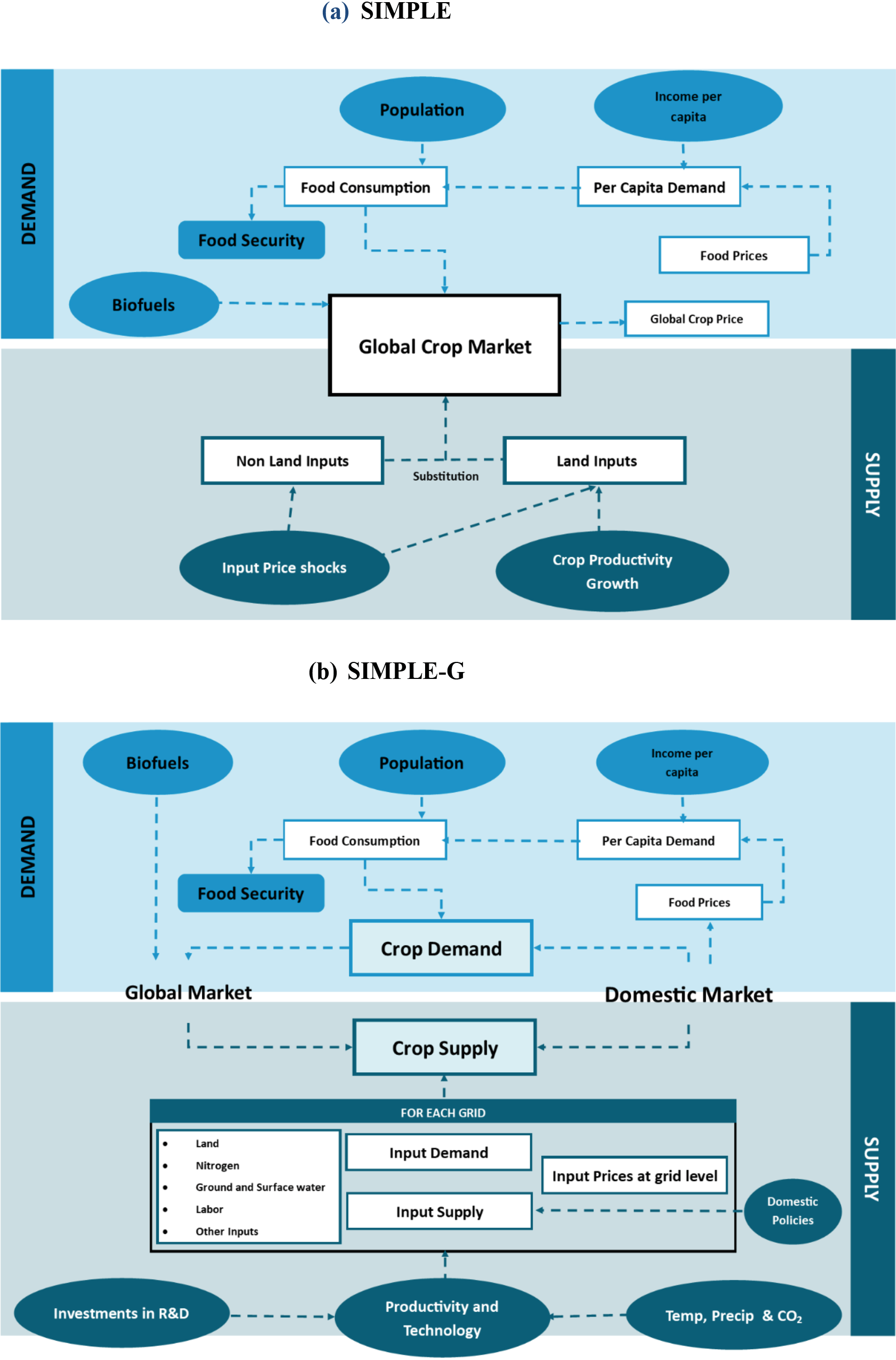
SIMPLE-G structure is built on SIMPLE but enabling crop production to be analysed at the grid level (Figure 1, panel b). Crop production in SIMPLE-G is no longer modelled at a world regional scale, but at a finer grid level.5 Since this model is georeferenced, it enables a more detailed representation of the various inputs used in crop production, such as land type, water use, and fertilizer application rates. Although this added complexity makes SIMPLE-G a more intricate variant of SIMPLE, both in modelling and scale, it also makes it a significantly more powerful analytical tool. First, it accounts for human systems’ responses to environmental changes, including adjustments in food consumption, agricultural production, land use, and water withdrawals, all influenced by shifts in market prices. Second, it offers a framework for measuring spillover effects transmitted between locations through market interactions. The ability to incorporate market-mediated effects and feedback loops between human and natural systems is, in fact, one of the advantages of SIMPLE-G over other traditional biophysical models (Hertel & Haqiqi, eds.). Another strength is the multi-scale approach used in SIMPLE-G that facilitates the connection between local-to-global changes, as presented in Figure 2. At the grid level, there could be a different composition of crop production, driven by differentiated contextual conditions (e.g., agroclimatic conditions). At the national, the overall quantity can be obtained by aggregating the grids’ amount based on assumptions about product differentiation. The procedure is the same to obtain world regional values, starting from aggregating national values. The greater the diversity of crops grown within a region, the lower the elasticity of substitution between these grid-based crop outputs.
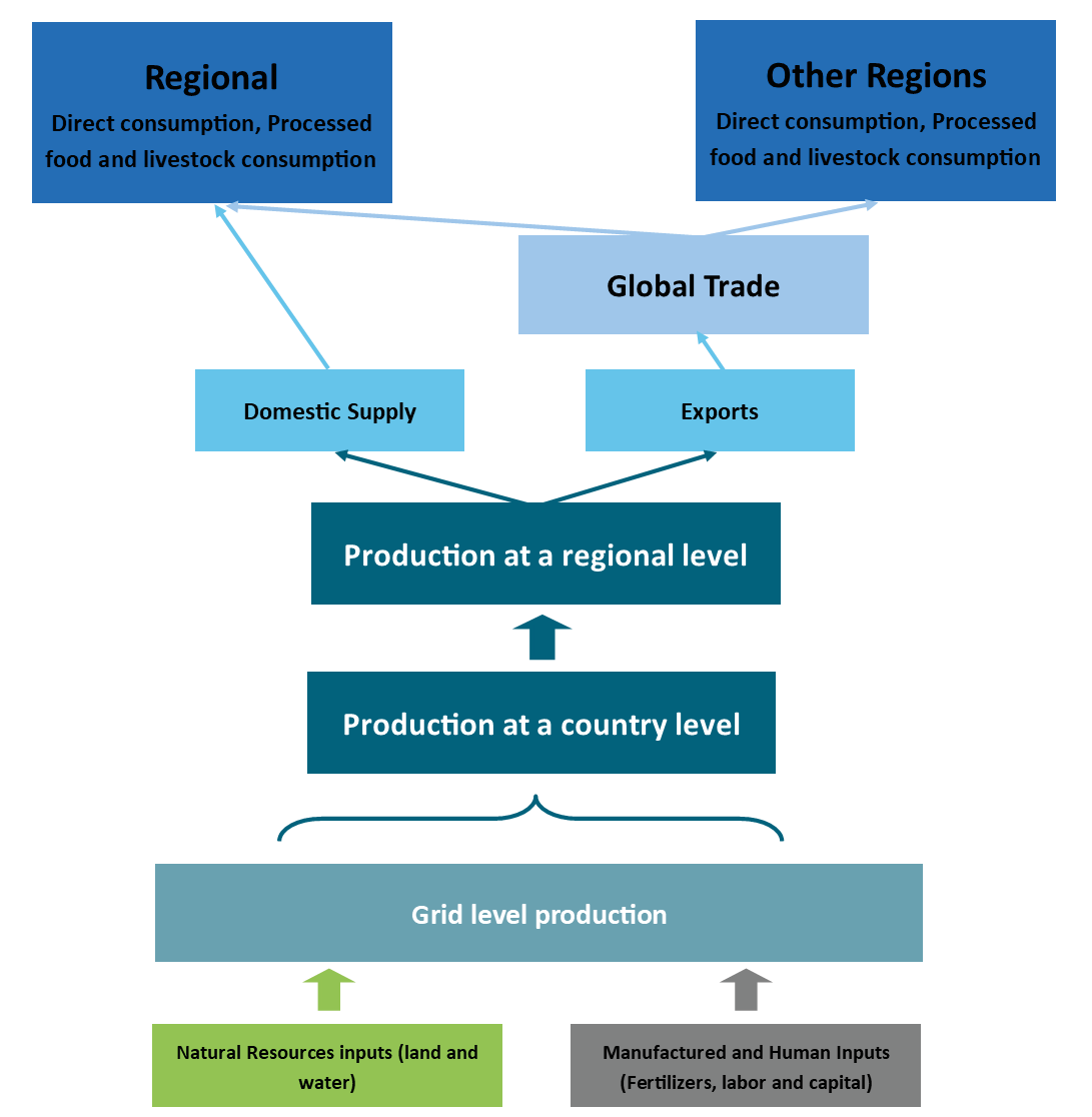
In this scenario, crop production can be supplied domestically (i.e., consumed within the country of origin) or exported. The decision to export or supply domestically depends on several factors, including the relative price of crops, which is influenced by production costs.
In this section, we describe the process followed to single out Italy from the macro-regional EU dataset, dividing the SIMPLE and SIMPLE-G world into 18 regions rather than 17 as in Baldos (2023b). The SIMPLE-G database follows, in fact, the structure and data of the SIMPLE model, but with Italy no more aggregated at the national level but rather subdivided into 5-arc-minute grids (the remaining 17 regions are aggregated) (Baldos et al., 2020b; Haqiqi et al., 2023b). The two databases were constructed separately but in tandem. To collect data, and in alignment with the Baldos (2023b) database, we referred, reviewed and processed various economic and biophysical information (Table 1).6 The benchmark primary data source was FAOSTAT, which provides different datasets at the national level (Table 2). However, FAOSTAT does not provide georeferenced data, so to create the SIMPLE-G model, we needed to consult the Earthstat database (Ramankutty et al., 2008). This database provides information on cropland, crop production, and fertilizer use by combining agricultural inventory data with satellite-derived land cover data, offering, thereby, information at a 5-minute (~10 km) spatial resolution.
| Dataset | Time span | Geographical Dimension | Links | ||||||||||||||||
|---|---|---|---|---|---|---|---|---|---|---|---|---|---|---|---|---|---|---|---|
| FAOSTAT | From 1961 to 2023 | Country level | https://www.fao.org/faostat/es/#data | ||||||||||||||||
| Earthstat | 2000 | 10km x10 km | http://www.earthstat.org/ | ||||||||||||||||
| ISIMIP | From 1861 to 2017 | 50 km x 50 km | https://www.isimip.org/ | ||||||||||||||||
| Agri4Cast | 1980-2022 / 2010 | 25 km x 25 km / 10 km x 10 km |
https://agri4cast.jrc.ec.europa.eu/DataPortal/Index.aspx | ||||||||||||||||
| AQUASTAT | 2005 | 10 km x 10 km | https://www.fao.org/aquastat/en/ | ||||||||||||||||
| GCWM | 1998-2002 | 10 km x 10 km | https://www.uni-frankfurt.de/45217988/Global_Crop_Water_Model__GCWM | ||||||||||||||||
| ISMEA Mercati | Up to 2024 | Italian regional level | https://www.ismea.it/mercati | ||||||||||||||||
| Italian Farm Accountancy Data Network (FADN) Rete di Informazione Contabile Agricola (RICA) |
2017 | Italian provincial level | https://rica.crea.gov.it/ | ||||||||||||||||
| Indagine Mercato Fondiario - CREA | Up to 2022 | Italian regional level | https://www.crea.gov.it/web/politiche-e-bioeconomia/-/indagine-mercato-fondiario | ||||||||||||||||
| Source: Own elaboration. | |||||||||||||||||||
| Dataset | Description | ||||||||||||||||||
|---|---|---|---|---|---|---|---|---|---|---|---|---|---|---|---|---|---|---|---|
| Production | Provides country-level data on crop and livestock production, including variables such as harvested area, production, yields, and animal stocks. | ||||||||||||||||||
| Population | Contains data on each country’s total population, disaggregated by gender and by rural and urban areas. | ||||||||||||||||||
| Macroeconomic Statistics | Offers country-level data on GDP, gross output, value added, and gross capital formation for land-intensive sectors and the food processing industry. | ||||||||||||||||||
| Land Use | Contains country data for crop area and value of agricultural production. | ||||||||||||||||||
| Prices | Presents prices for all crops and livestock at a country level. | ||||||||||||||||||
| Source: Own elaboration. | |||||||||||||||||||
The Earthstat database was used to determine the structural base of the SIMPLE-G model, meaning the number of grids of the model. In doing so, we followed the construction of SIMPLE-G Brazil (Wang et al., 2022a), wherein crop production estimates are formulated by considering only the top 80% of the most significant crops in the country. This approach helps eliminate potential statistical errors associated with minor crop estimates from Earthstat (Ramankutty et al., 2008).7
The final database is composed of 3,745 grids, which exhibited both cropland and agricultural output (Table 3).
| Number of grids | Output | ||||||||||||||||||
|---|---|---|---|---|---|---|---|---|---|---|---|---|---|---|---|---|---|---|---|
| 0 | >0 | ||||||||||||||||||
| Cropland | 0 | 346 | 328 | ||||||||||||||||
| >0 | 396 | 3745 | |||||||||||||||||
| Source: Own elaboration. | |||||||||||||||||||
However, information coming from Earthstat needs to be historically validated. To do that, we used data provided by the Inter-Sectoral Impact Model Intercomparison Project (ISIMIP), which consists of a time-varying historical land-use (LU) dataset including various land-use categories such as pastures, rangeland, and five distinct crop types.8
The ISIMIP’s geographical coverage is lower than Earthstat’s, and the geographical disaggregation is less fine (50 km by 50 km grid dimension), which is why we decided to consider Earthstat’s data in the model. The same applies to crop data from the Agri4Cast toolbox (25 km by 25 km grid dimension). Although the irrigation data available in the toolbox has a grid dimension equal to the one used (10 km by 10 km), it is outdated, corresponding to 2010, and lacks information on rainfed land.
Given the current extreme relevance of water issues in the SIMPLE-G database for Italy, we decided to include the water model, following Haqiqi et al. (2023b). This extension allows for the estimation of local demand for agricultural water for irrigation water, which is crucial to modelling the impacts of sustainability policies and climate change shocks. These external events can have, in fact, different effects on irrigated versus non-irrigated (i.e., rainfed) crops due to their varying responses to heat and water stress.
This approach means that within each grid cell, two distinct production functions, rainfed and irrigated crops, compete for irrigable land.
Regarding data on water, we started collecting information from AQUASTAT (source: FAO), a global information system focused on hydric resources and agricultural water management. AQUASTAT provides georeferenced information at a 5-minute (~10 km) spatial resolution. Information on irrigated and rainfed hectares came from the Global Crop Water Model (GCWM) database, developed by Siebert & Döll (2008) within a 5-minute (~10 km) grid dimension. In addition, to obtain information on prices and values of irrigated vs non-irrigated land and crops, we consulted the Italian Farm Accountancy Data Network9 (FADN).10
Another option for estimating crop prices in Italy is using data provided by ISMEA (Instituto di Servizi per il mercato agricolo alimentare), which represent market prices from the most representative local markets specific to product varieties and sales conditions.11
However, reliance on this dataset could lead to misleading estimates, given that the dataset provides prices differentiated for crops and regions rather than an aggregated crop price, as needed for the models. SIMPLE and SIMPLE-G models lack, in fact, differentiation among various crops. In addition, prices are provided only for specific groups of crops, differentiated by regions, which are those crops considered the most relevant for the regional agricultural economic output. This dataset is not, therefore, suitable to generate a representative and comparable regional aggregate crop price, as requested by the model, generating potential estimation biases.
Finally, we need data on the land market, collected from the dataset provided by the Council for Agricultural Research and Economics (CREA), to define the average farmland values at regional and national levels.
To sum up, by utilizing the dataset mentioned above and applying the parameters provided by Baldos (2023b) regarding country-specific production shares in global and local markets, as well as income and price elasticities, we were able to build a new database for SIMPLE with 18 regions, specifically distinguishing Italy. For both SIMPLE and SIMPLE-G models, the base year is 2017. The choice of the base year is mainly due to the availability of data that would enable the construction of a coherent dataset for both SIMPLE and SIMPLE-G.
Table 4 presents the estimated values for Italy in 2017 alongside the aggregate values for the remaining 17 regions, covering the key variables required for the model.
| Variable | Italy | Other Regions | |||||||||||||||||
|---|---|---|---|---|---|---|---|---|---|---|---|---|---|---|---|---|---|---|---|
| Income per capita (in USD) | 31,509 | 278,783 | |||||||||||||||||
| Population (in 1000 person) | 60,004 | 7,524,960 | |||||||||||||||||
| Crop Use: Regional Biofuels (in 1000 Mt: Corn Eq) | 3,013 | 447,499 | |||||||||||||||||
| Crop Output (in 1000 MT: corn-eq) | 132,549 | 12,789,222 | |||||||||||||||||
| Value of Crop Output (in 1000 usd) | 29,028,232 | 2,800,839,581 | |||||||||||||||||
| Cropland cover (in 1000 ha) | 9,218 | 1,557,064 | |||||||||||||||||
| Value of Cropland (in 1000 usd) | 4,830,646 | 540,050,675 | |||||||||||||||||
| Value of Non-Land Inputs (in 1000 usd) | 24,197,586 | 2,260,788,898 | |||||||||||||||||
| Crop Use: Livestock sector (in 1000 Mt: Corn Eq.) | 32,450 | 2,538,728 | |||||||||||||||||
| Crop Use: Food processing sector (in 1000 Mt: Corn Eq.) | 37,698 | 3,100,306 | |||||||||||||||||
| Source: Own elaboration based on FAOSTAT and Baldos (2023b). | |||||||||||||||||||
3.1. Database illustration and calibration
Figure 3 illustrates the 3,745 grids with cropland and crop production in Italy obtained from Earthstat database.
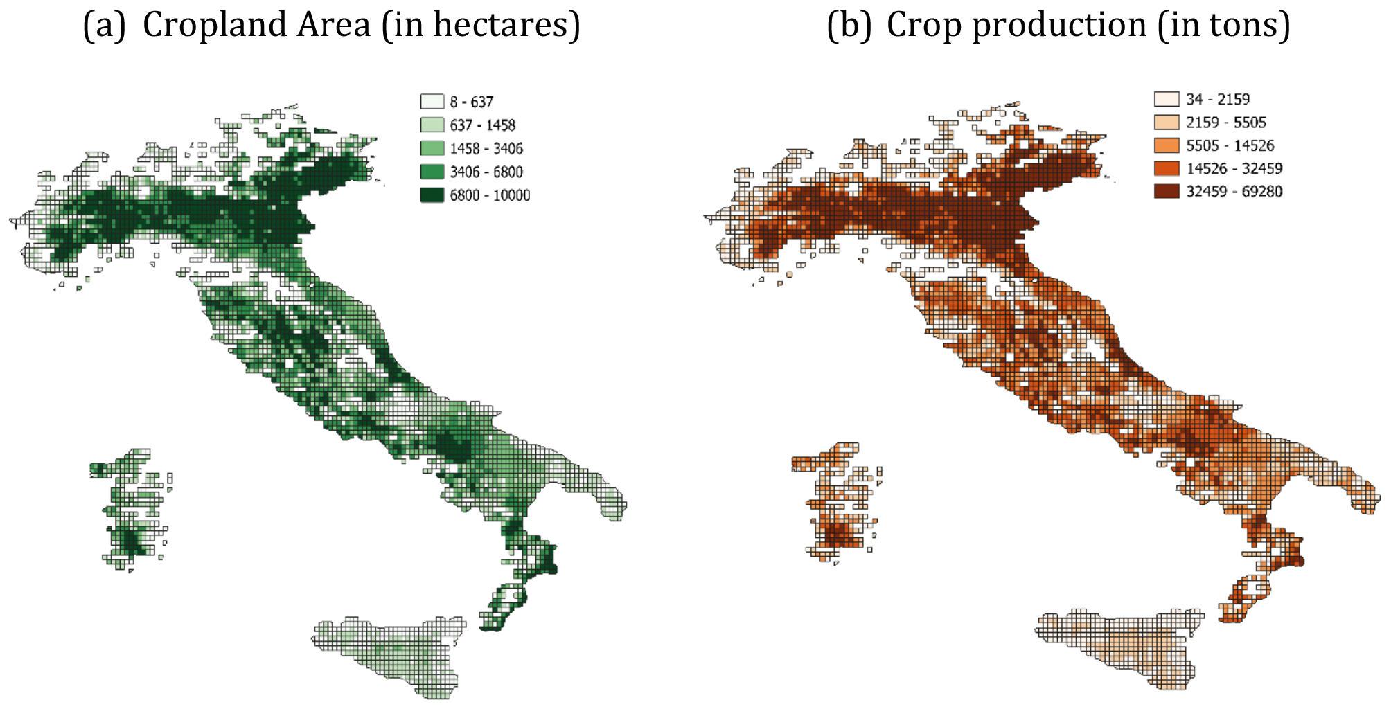
The data populating the Italian dataset come from the data sources described in the previous section, and they are better discussed and visualised here.
A first group of variables refers to environmental issues: nitrogen and water use.
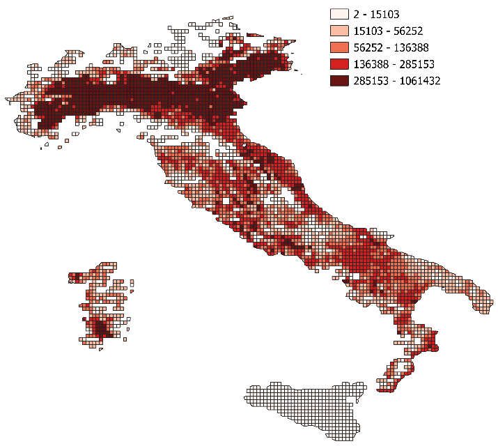
The SIMPLE-G model considers nitrogen fertilizers as one of the key inputs of production function, and, therefore, the amount of nitrogen applications in each grid is needed to calibrate the base year. To achieve this, we used the Earthstat database, which collects national and sub-national data on fertilizer application rates for crops and crop groupings from the National Institute of Statistics (ISTAT). Figure 4 depicts the distribution across Italy depicting a more intensive use in the northern part of the country, which aligns with results obtained for cropland area and production.
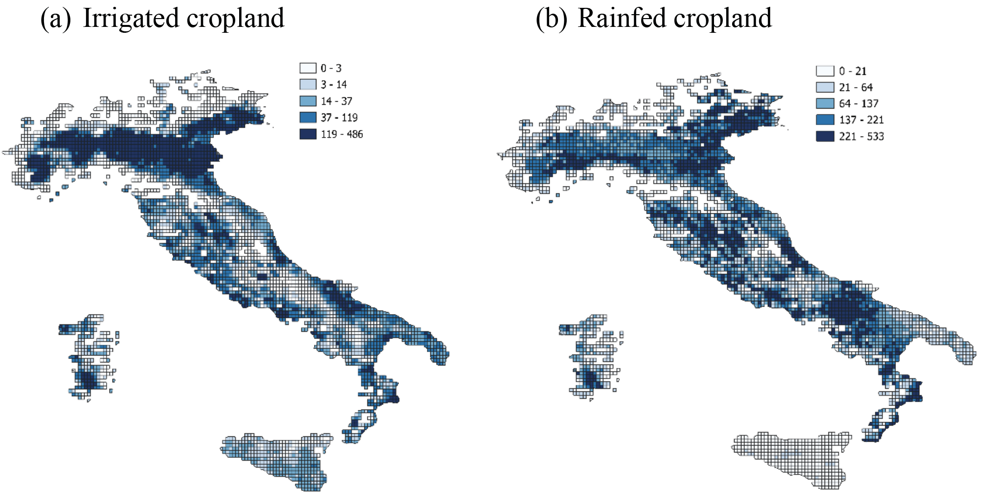
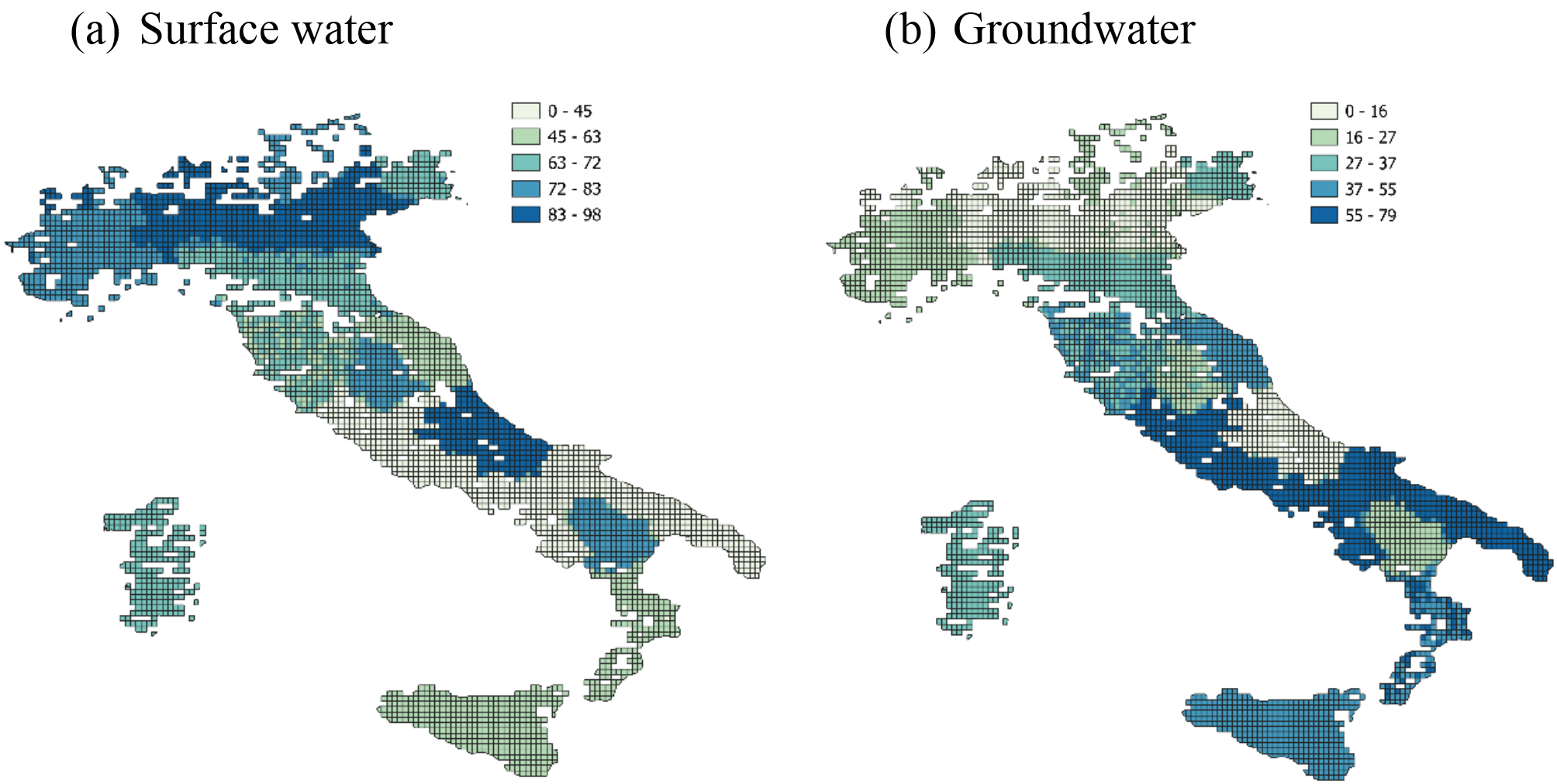
In the case of water use, SIMPLE-G model incorporates rainfed and irrigated water use as critical inputs for crop production, differentiating between irrigated and rainfed crop supply. In addition, in the irrigated crop production function, the demand for water is subdivided into groundwater and surface water. Figure 5 shows the distribution of irrigated (panel a) and rainfed (panel b) cropland hectares in each grid (source: GCWM), while Figure 6 depicts the gridded distribution of irrigated land through groundwater (panel a) and surface water (panel b) (source: AQUASTAT).12
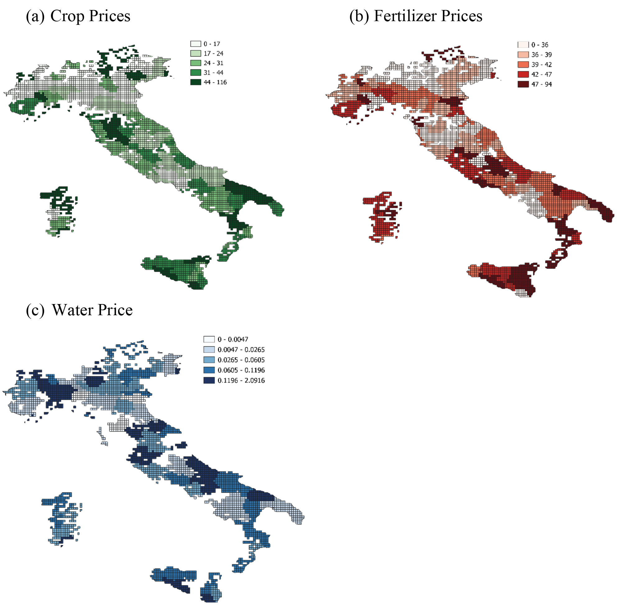
Regarding economic variables, the model needs price information, specifically on land, crop, fertilizers and water prices. To estimate the prices of crops and fertilizers, we used the Italian FADN database at the NUTS3 level and considered the ratio between values and volumes (Figure 7). In estimating crop (panel a) and fertilizer (panel b) prices, to be faithful to Earthstat database, we considered crops included in the 80% of total production. In the case of water (panel c), prices were also calculated starting from the Italian FADN data on total water use in m3.13
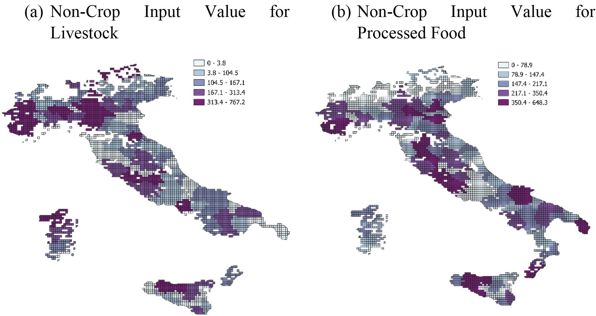
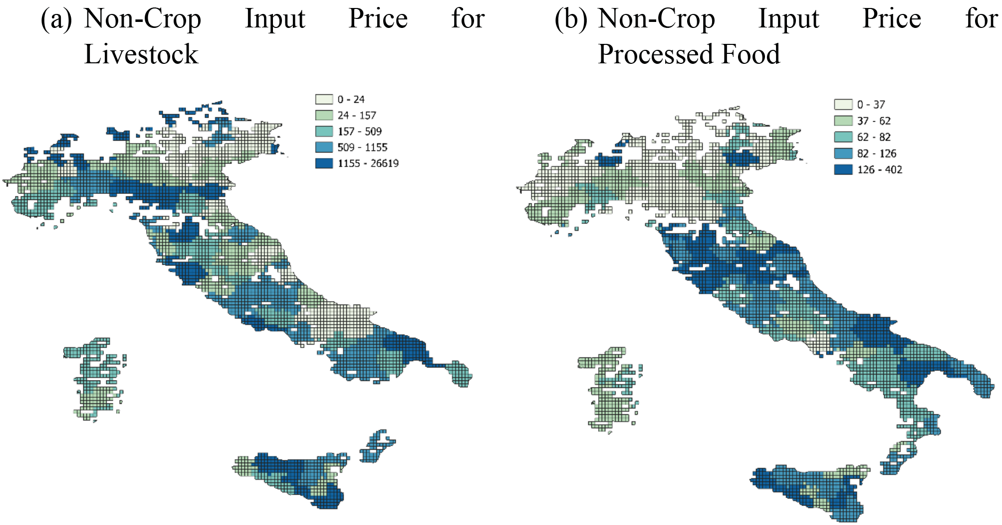
We also extracted data on farmers’ expenses from the Italian FADN database to estimate the prices and values of non-crop inputs for livestock and processed food (Figure 8 and Figure 9).14 To calculate the total value of non-crop inputs, we considered water, electricity, fuels, veterinary and machinery expenses, commercial and processing expenses, general and land expenses, and salaries. The total values obtained were then divided by their corresponding quantities, distinguishing between the two types of activities to obtain prices.15
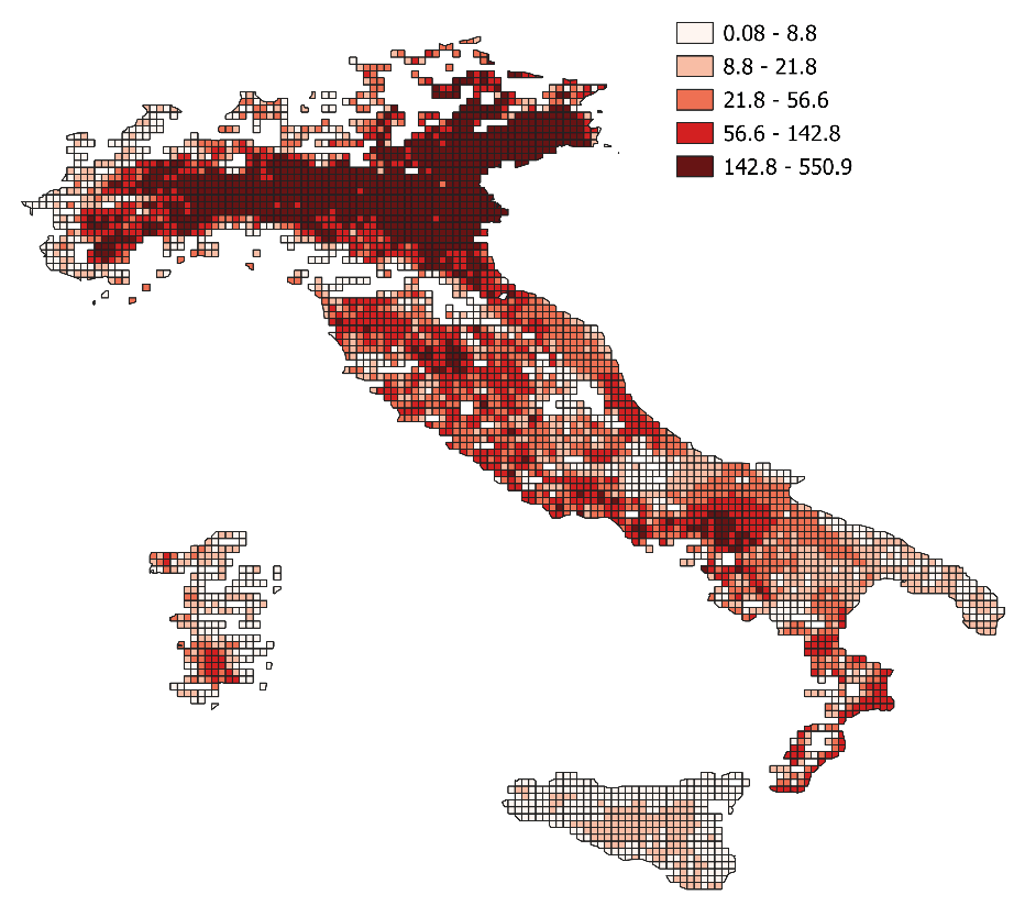
Finally, calibrating the SIMPLE-G model requires determining the cropland values at a grid level. As anticipated in the previous section, we collected data from the CREA’s land market database (Indagine-mercato-fondiario) and downscaled them at the grid level (Figure 10). To do so, we have assumed that all cropland has a uniform value (expressed in euros per hectare) within a NUTS2 (Italian region) area.16
To ensure time consistency, a final note should be made regarding treating the datasets above. In addition, since most georeferenced datasets are based between 2000 and 2005, it was necessary to update them to 2017 by rescaling the geospecial structures to the values provided by FAOSTAT.
3.2. Estimation of the drivers of the model
The last step was to estimate the main driver variables needed to simulate a baseline scenario to 2030 for both the SIMPLE and SIMPLE-G models, with Italy as a single country. This scenario will serve as the basis for additional simulations.
Population growth rates were derived using the population projections developed by Samir & Lutz (2017), while GDP per capita estimates were based on projections by Crespo Cuaresma (2017). These projections follow the intermediate Shared Socioeconomic Pathway (SSP2) the International Institute for Applied Systems Analysis (IIASA) created. Regarding future biofuel demand, they were constructed using estimates provided by IEA (2024). The adoption of these databases aligns with the methodology proposed by SIMPLE modellers in Baldos et al. (2020b), Haqiqi et al. (2023b), and Baldos (2023b). For the TFP, econometric estimations were performed using a time series model to forecast output and input data for 2030 based on a panel data structure (see Annex I for details).
Table 5 presents the percentage variations of each variable between 2017 and 2030.
| Population | GDP per capita | Biofuels demand | TFP | ||||||||||||||||
|---|---|---|---|---|---|---|---|---|---|---|---|---|---|---|---|---|---|---|---|
| AUS_NZ | 22.01 | 40.92 | 6.67 | -0.5 | |||||||||||||||
| BRA | 9.68 | 38.59 | 97.74 | 18.7 | |||||||||||||||
| CAN | 15.41 | 29.57 | 64.23 | 13.3 | |||||||||||||||
| CC_AMER | 13.48 | 41.23 | 58.33 | 0.9 | |||||||||||||||
| CHINA | 1.32 | 126.32 | 19.56 | 10.3 | |||||||||||||||
| C_ASIA | 30.61 | 334.19 | 224.75 | 30.2 | |||||||||||||||
| EU | 4.26 | 39.46 | 52.86 | 7.1 | |||||||||||||||
| E_EURO | -1.97 | 59.91 | 0.00 | 20.9 | |||||||||||||||
| ITA | 0.77 | 69.70 | 103.38 | 1.7 | |||||||||||||||
| JPN_KR | -1.92 | 9.03 | 224.75 | 3.9 | |||||||||||||||
| M_EAST | 22.40 | 30.12 | 331.03 | 18.3 | |||||||||||||||
| N_AFR | 17.28 | 33.27 | 0.00 | 48.3 | |||||||||||||||
| SE_ASIA | 12.15 | 100.20 | 224.75 | 4.3 | |||||||||||||||
| SSA | 38.17 | 67.84 | 16243.201 | 15.9 | |||||||||||||||
| S_AFR | 11.90 | 49.55 | 0.00 | 15.2 | |||||||||||||||
| S_AMER | 13.51 | 46.24 | 58.33 | 10.8 | |||||||||||||||
| S_ASIA | 17.80 | 144.12 | 0.00 | 18.2 | |||||||||||||||
| US | 11.83 | 20.83 | 24.29 | 10.1 | |||||||||||||||
| 1 Note: Estimates for the Sub-Saharan Africa region was unavailable in the IEA (2024) database. Hence, this projection was taken from Baldos (2023b). | |||||||||||||||||||
| Source: Own elaboration. | |||||||||||||||||||
4. A first application of SIMPLE-IT
In the case of SIMPLE, the Italian database has already been properly structured for integration into the GEMPACK software, and the model is ready to be tested. As a first application, we conducted a baseline simulation to evaluate the expected impacts of the evolution of population, GDP per capita, biofuel demand and crop TFP on agricultural production and land use at the national level projected to 2030. Table 6 presents the results showing the percentage impact on crop prices, highlighting the contribution of each driver to the total effect. As shown, the estimated baseline has an overall negative impact on global crop prices (-6.36%) and in most regions, indicating that prices would decrease under the given scenario. This can be explained by the fact that although demand-side drivers (population growth, GDP per capita, and biofuels) exert upward pressure on prices due to increased crop demand (8.85% from population growth, 7.38% from GDP per capita, and 1.32% from biofuels), this effect is more than offset by improvements in sector productivity. Overall, the rise in productivity leads to a global price reduction of 17.21%, increasing production enough to counterbalance the higher demand.
| Total Effect | Population | GDP per capita | Biofuels Demand | Crop TFP | |||||||||||||||
|---|---|---|---|---|---|---|---|---|---|---|---|---|---|---|---|---|---|---|---|
| AUS_NZ | -1.23 | 8.19 | 2.11 | 0.91 | -12.43 | ||||||||||||||
| BRA | -7.64 | 5.39 | 3.08 | 3.62 | -19.73 | ||||||||||||||
| C_Asia | -4.15 | 14.17 | 12.94 | 0.42 | -31.68 | ||||||||||||||
| CAN | -6.26 | 6.47 | 2.86 | 1.62 | -17.22 | ||||||||||||||
| CC_Amer | -1.53 | 7.05 | 3.31 | 0.98 | -12.87 | ||||||||||||||
| CHINA | -7.81 | 1.83 | 4.56 | 0.25 | -14.45 | ||||||||||||||
| E_Euro | -12.57 | 3.23 | 3.24 | 0.65 | -19.70 | ||||||||||||||
| EU | -6.57 | 5.49 | 2.30 | 1.17 | -15.53 | ||||||||||||||
| ITA | -4.62 | 4.12 | 1.34 | 1.56 | -11.64 | ||||||||||||||
| JPN_KR | -6.77 | 3.05 | 1.94 | 0.70 | -12.46 | ||||||||||||||
| M_East | -8.12 | 9.68 | 2.06 | 0.54 | -20.39 | ||||||||||||||
| N_Afr | -20.20 | 8.53 | 3.47 | 0.57 | -32.77 | ||||||||||||||
| S_Afr | -6.96 | 6.50 | 3.62 | 0.75 | -17.83 | ||||||||||||||
| S_Amer | -5.40 | 6.85 | 3.24 | 0.88 | -16.38 | ||||||||||||||
| S_Asia | -1.85 | 10.74 | 10.47 | 0.19 | -23.25 | ||||||||||||||
| SE_Asia | 6.91 | 7.74 | 8.39 | 0.50 | -9.72 | ||||||||||||||
| SSA | 7.82 | 18.89 | 5.41 | 5.88 | -22.36 | ||||||||||||||
| US | -5.33 | 5.49 | 1.91 | 3.85 | -16.59 | ||||||||||||||
| WORLD | -6.36 | 6.33 | 3.40 | 1.12 | -17.21 | ||||||||||||||
| Source: Own elaboration. | |||||||||||||||||||
Table 7 illustrates the impact of the simulation on crop production, breaking down the total impact by and the total effect of each driver in the model. Analysing the contribution of productivity changes to agricultural output, it is evident that productivity growth leads to an overall global production increase (6.54%). However, in some regions, production declines due to lower comparative competitiveness, as seen in Italy, where production decreased by 9.17%. Regarding demand-side drivers, all have a positive impact, as expected, with global effects of 8.73% from population growth, 6.19% from GDP per capita, and 1.82% from biofuels.
| Total Effect | Population | GDP per capita | Biofuels Demand | Crop TFP | |||||||||||||||
|---|---|---|---|---|---|---|---|---|---|---|---|---|---|---|---|---|---|---|---|
| AUS_NZ | -2.65 | 10.22 | 2.63 | 1.13 | -16.63 | ||||||||||||||
| BRA | 33.45 | 8.30 | 4.63 | 5.55 | 14.97 | ||||||||||||||
| C_Asia | 69.06 | 22.54 | 18.90 | 0.67 | 26.94 | ||||||||||||||
| CAN | 22.58 | 9.71 | 4.19 | 2.43 | 6.24 | ||||||||||||||
| CC_Amer | 0.20 | 7.67 | 3.59 | 1.07 | -12.14 | ||||||||||||||
| CHINA | 12.26 | 2.14 | 5.19 | 0.29 | 4.65 | ||||||||||||||
| E_Euro | 29.49 | 4.91 | 4.77 | 0.99 | 18.82 | ||||||||||||||
| EU | 7.17 | 6.42 | 2.66 | 1.37 | -3.27 | ||||||||||||||
| ITA | -1.56 | 4.48 | 1.44 | 1.69 | -9.17 | ||||||||||||||
| JPN_KR | 0.90 | 2.92 | 1.85 | 0.67 | -4.55 | ||||||||||||||
| M_East | 30.75 | 13.91 | 2.89 | 0.77 | 13.19 | ||||||||||||||
| N_Afr | 70.17 | 10.43 | 4.08 | 0.70 | 54.97 | ||||||||||||||
| S_Afr | 25.32 | 9.19 | 5.01 | 1.06 | 10.06 | ||||||||||||||
| S_Amer | 16.98 | 8.80 | 4.10 | 1.13 | 2.95 | ||||||||||||||
| S_Asia | 38.31 | 13.57 | 12.80 | 0.24 | 11.69 | ||||||||||||||
| SE_Asia | 16.57 | 8.27 | 8.89 | 0.53 | -1.12 | ||||||||||||||
| SSA | 48.75 | 24.93 | 7.02 | 7.75 | 9.06 | ||||||||||||||
| US | 15.56 | 7.09 | 2.43 | 4.98 | 1.06 | ||||||||||||||
| WORLD | 23.28 | 8.73 | 6.19 | 1.82 | 6.54 | ||||||||||||||
| Source: Own elaboration. | |||||||||||||||||||
Table 8 and Table 9 present the results of cropland use, regarding hectares and land prices. As observed, demand-side drivers increase the need for cropland to meet rising crop demand, leading to a global increase of 7.44% in land use. This, in turn, creates upward pressure on land prices. However, once again, productivity improvements introduce a compensatory effect. As the sector becomes more productive, fewer hectares are required to achieve the same production level, resulting in a global reduction of 2.59% in land use. Although this mitigates the need for additional land, it does not fully offset it, leading to a net global increase of 4.86% in land use. At the regional level, however, some areas fully compensate for demand-side drivers through productivity gains – for example, in Italy, where total land use decreases by 0.44%.
| Total Effect | Population | GDP per capita | Biofuels Demand | Crop TFP | |||||||||||||||
|---|---|---|---|---|---|---|---|---|---|---|---|---|---|---|---|---|---|---|---|
| AUS_NZ | -1.16 | 5.48 | 1.41 | 0.61 | -8.65 | ||||||||||||||
| BRA | 6.38 | 3.89 | 2.20 | 2.61 | -2.32 | ||||||||||||||
| C_Asia | 15.68 | 10.17 | 9.04 | 0.30 | -3.84 | ||||||||||||||
| CAN | 2.24 | 2.48 | 1.09 | 0.62 | -1.96 | ||||||||||||||
| CC_Amer | -0.22 | 2.47 | 1.16 | 0.34 | -4.19 | ||||||||||||||
| CHINA | 0.58 | 0.66 | 1.63 | 0.09 | -1.79 | ||||||||||||||
| E_Euro | 3.76 | 2.35 | 2.32 | 0.47 | -1.38 | ||||||||||||||
| EU | 0.01 | 0.82 | 0.34 | 0.18 | -1.33 | ||||||||||||||
| ITA | -0.44 | 0.61 | 0.19 | 0.23 | -1.47 | ||||||||||||||
| JPN_KR | -0.44 | 0.44 | 0.28 | 0.10 | -1.25 | ||||||||||||||
| M_East | 1.25 | 1.51 | 0.32 | 0.08 | -0.66 | ||||||||||||||
| N_Afr | 2.30 | 1.31 | 0.52 | 0.09 | 0.38 | ||||||||||||||
| S_Afr | 2.53 | 2.45 | 1.36 | 0.28 | -1.56 | ||||||||||||||
| S_Amer | 3.12 | 4.67 | 2.20 | 0.60 | -4.35 | ||||||||||||||
| S_Asia | 5.28 | 3.83 | 3.71 | 0.07 | -2.33 | ||||||||||||||
| SE_Asia | 3.81 | 2.61 | 2.83 | 0.17 | -1.80 | ||||||||||||||
| SSA | 15.53 | 12.64 | 3.60 | 3.93 | -4.64 | ||||||||||||||
| US | 1.48 | 2.02 | 0.70 | 1.42 | -2.65 | ||||||||||||||
| WORLD | 4.86 | 4.15 | 2.25 | 1.04 | -2.59 | ||||||||||||||
| Source: Own elaboration. | |||||||||||||||||||
| Total Effect | Population | GDP per capita | Biofuels Demand | Crop TFP | |||||||||||||||
|---|---|---|---|---|---|---|---|---|---|---|---|---|---|---|---|---|---|---|---|
| AUS_NZ | -2.05 | 9.76 | 2.51 | 1.08 | -15.40 | ||||||||||||||
| BRA | 11.68 | 7.13 | 4.02 | 4.78 | -4.25 | ||||||||||||||
| C_Asia | 29.70 | 19.47 | 17.00 | 0.58 | -7.36 | ||||||||||||||
| CAN | 8.22 | 9.15 | 3.99 | 2.29 | -7.21 | ||||||||||||||
| CC_Amer | -0.80 | 8.81 | 4.13 | 1.23 | -14.96 | ||||||||||||||
| CHINA | 2.09 | 2.39 | 5.87 | 0.32 | -6.49 | ||||||||||||||
| E_Euro | 6.82 | 4.26 | 4.21 | 0.86 | -2.51 | ||||||||||||||
| EU | 0.08 | 7.48 | 3.11 | 1.60 | -12.11 | ||||||||||||||
| ITA | -3.91 | 5.42 | 1.75 | 2.05 | -13.13 | ||||||||||||||
| JPN_KR | -3.93 | 3.90 | 2.48 | 0.90 | -11.22 | ||||||||||||||
| M_East | 11.92 | 14.44 | 3.03 | 0.80 | -6.35 | ||||||||||||||
| N_Afr | 22.96 | 13.09 | 5.21 | 0.88 | 3.79 | ||||||||||||||
| S_Afr | 9.32 | 9.06 | 4.99 | 1.05 | -5.78 | ||||||||||||||
| S_Amer | 5.64 | 8.45 | 3.97 | 1.09 | -7.86 | ||||||||||||||
| S_Asia | 20.17 | 14.76 | 14.11 | 0.27 | -8.97 | ||||||||||||||
| SE_Asia | 14.28 | 9.83 | 10.60 | 0.63 | -6.78 | ||||||||||||||
| SSA | 29.42 | 23.98 | 6.80 | 7.46 | -8.82 | ||||||||||||||
| US | 5.40 | 7.36 | 2.54 | 5.17 | -9.67 | ||||||||||||||
| WORLD | 10.33 | 8.85 | 7.38 | 1.32 | -7.22 | ||||||||||||||
| Source: Own elaboration. | |||||||||||||||||||
The changes in land use also explain the observed impact on land prices, which increase globally by 10.33%. Since higher land demand drives prices up (with demand-side drivers contributing to a 17.55% global price increase), productivity improvements are unable to fully counteract this effect. While productivity growth reduces land prices by 7.22%, it is not enough to fully offset the upward pressure generated by demand-side factors.
External shocks, such as climate change and extreme events, are shaping the sustainability of the agricultural and agrifood sectors worldwide, and this will become even more relevant due to climate scenario projections. Tools for ex-ante analyses are becoming increasingly crucial to understanding how policy design should evolve to address future challenges, such as international competitiveness and food security. In this context, this paper provides, for the first time, the scientific community with the extension of SIMPLE and SIMPLE-G models to a European country, Italy.
The paper not only describes the models, discusses the related literature, and documents the work performed to create the database for a new country but also presents: (i) the estimated values used to calibrate the baseline (in both models for 2017); (ii) the exogenous driver projections extending to 2030; (iii) a fist application of SIMPLE- IT model.
The first application of SIMPLE, integrating for Italy, presented in Section 4, demonstrated that agricultural production is projected to increase due to the included drivers (demand and productivity). The observed reduction in production in certain regions, such as Italy, is primarily explained by the lower productivity gains in comparison to the other regions, leading to a reallocation of production toward these regions. The overall increase in global crop production is associated with a reduction in agricultural prices.
Regarding land use, the results exhibit a similar pattern: an increase in the utilized area, except in regions where production decreased or where the increase was negligible. Higher agricultural productivity reduces the land requirements to achieve equivalent production levels. However, the rise in demand for agricultural products drives additional production, which in turn requires more land. This explains the increase in utilized hectares, although at a lower rate than the growth in production. Moreover, agricultural land prices exhibit an upward trend because of increased demand.
Additional steps are required to validate the SIMPLE-G model presented in this paper before running simulations. Specifically, grid-level elasticities of substitution should be defined in the model, following the methodology employed by Haqiqi et al. (2023b). Once this validation is completed, the model will be ready to conduct location-specific simulations, such as assessing the impacts of local climatic events or policy interventions. Both SIMPLE and SIMPLE-G models can be, in fact, used to simulate policy-oriented shocks, such as changes in agricultural land exploitation, agricultural water use (wastewater), water management strategies (i.e., collective vs private) or in farming processing (e.g., organic). The models incorporate, in fact, market-mediated effects and feedback loops between human and natural systems, guiding heterogeneous economic decisions at different spatial levels (national for SIMPLE while gridded for SIMPLE-G). They provide a framework for measuring spillover effects transmitted across locations through markets and accounts for tele-coupling distant regions, enabling the analysis of interregional dependencies on a local-global scale. The capacity of SIMPLE-G to capture interactions is one of the main strengths of this model, especially for policy design (Baldos et al., 2020b). Overall, the several potential applications of both of these models will provide unique insights for sustainable policy targeting at the local, national and global levels (Hertel & Haqiqi, eds.). Today, the issue is more relevant than ever, given the current vibrant debate on what will come after the 2030 Agenda goals and how to plan sustainable development trajectories in the future within an anticipatory governance framework.
Authors would like to thank all the participants of the 13th AIEAA Conference who attended the Organised Session “Integrating Water and Ecosystem Services into Economic Models: insight from the RUEESnexus and MUST4water projects”. Special thanks go to Arianna di Paola (National Research Council of Ital, Institute for BioEconomy), the SIMPLE research group at Purdue University (US), and the CREA researchers for their suggestions.
This work was funded by the Next Generation EU – Italian National Recovery and Resilience Plan (NRRP), Mission 4, Component C2, Investment 1.1, “Fondo per il Programma Nazionale di Ricerca e Progetti di Rilevante Interesse Nazionale (PRIN)” (Directorial Decree n. 2022/1409) - under the project ʺMUlti-scale modelization toward Socio-ecological Transition for Water management (MUST4Water) ʺ, n. P2022R8ZTW. This work reflects only the authorsʹ views and opinions, neither the Ministry for University and Research nor the European Commission.
This work is also part of ACT4CAP27, which is funded by the European Union. Horizon Europe Grant Agreement No. 101134874. Views and opinions expressed are however those of the authors only and do not necessarily reflect those of the European Union or the European Commission. Neither the European Union nor the granting authority can be held responsible for them.
Ackerberg, D., Benkard, C. L., Berry, S., & Pakes, A. (2007). Econometric tools for analyzing market outcomes. Handbook of Econometrics, vol. 6A, ed. J. J. Heckman and E. Leamer, 4172–4276. Amsterdam: Elsevier.
Baldos, U. L. C. (2023a). Impacts of US Public R&D Investments on Agricultural Productivity and GHG Emissions. Journal of Agricultural and Applied Economics, 55(3), 536-550.
Baldos, U. L. (2023b). SIMPLE Database and Model for Base Year 2017. MyGeoHUB.
Baldos, U. L. C., Fuglie, K. O., & Hertel, T. W. (2020a). The research cost of adapting agriculture to climate change: A global analysis to 2050. Agricultural Economics, 51(2), 207-220
Baldos, U. L. C., Haqiqi, I., Hertel, T. W., Horridge, M., & Liu, J. (2020b). SIMPLE-G: A multiscale framework for integration of economic and biophysical determinants of sustainability. Environmental Modelling & Software, 133, 104805.
Baldos, U. L. C., & Hertel, T. W. (2013). Looking back to move forward on model validation: Insights from a global model of agricultural land use. Environmental Research Letters, 8(3), 034024.
Baldos, U. L. C., & Hertel, T. W. (2014). Global Food Security in 2050: The Role of Agricultural Productivity and Climate Change. Political Economy - Development: Environment Journal.
Baldos, U. L. C., & Hertel, T. W. (2015). The role of international trade in managing food security risks from climate change. Food Security, 7(2), 275-290.
Crespo Cuaresma, J. (2017). Income projections for climate change research: A framework based on human capital dynamics, Global Environmental Change, Volume 42, Pages 226-236, ISSN 0959-3780.
Dorfman, J. H., Irwin, S. H., Gopinath, M., & Zilberman, D. (2024). The future of agricultural and applied economics departments. Applied Economic Perspectives and Policy, 46(3), 834-844.
Fuglie, K., Ray, S., Baldos, U. L. C., & Hertel, T. W. (2022). The R&D cost of climate mitigation in agriculture. Applied Economic Perspectives and Policy, 44(4), 1955-1974.
Haqiqi, I., Grogan, D. S., Bahalou Horeh, M., Liu, J., Baldos, U. L., Lammers, R., & Hertel, T. W. (2023a). Local, regional, and global adaptations to a compound pandemic-weather stress event. Environmental Research Letters, 18(3).
Haqiqi, I., Bowling, L., Jame, S., Baldos, U., Liu, J., & Hertel, T. (2023b). Global drivers of local water stresses and global responses to local water policies in the United States. Environmental Research Letters, 18(6), 065007.
Haqiqi, Iman and Thomas W. Hertel (eds.) SIMPLE-G: A Gridded Economic Approach to Analysis of Sustainability of the Earth’s Land and Water Resources, Springer International Publishing Switzerland, 2025. https://doi.org/10.1007/978-3-031-68054-0
Hertel, B. T. W., Baldos, U. L. C., & Fuglie, K. O. (2020). Trade in technology: A potential solution to the food security challenges of the 21st century. European Economic Review, 127, 103479. https://doi.org/10.1016/j.euroecorev.2020.103479
Hertel, T. W., Ramankutty, N., & Baldos, U. L. C. (2014). Global market integration increases likelihood that a future African Green Revolution could increase crop land use and CO2 emissions. Proceedings of the National Academy of Sciences, 111(38), 13799-13804.
Hertel, T. W. (2018). Economic perspectives on land use change and leakage. Environmental Research Letters, 13(7), 075012.
IEA (2024), Renewable Energy Progress Tracker, IEA, Paris https://www.iea.org/data-and-statistics/data-tools/renewable-energy-progress-tracker
Kabir, K., Baldos, U. L. C., & Hertel, T. W. (2023). The new Malthusian challenge in the Sahel: Prospects for improving food security in Niger. Food Security, 15(2), 455-476. https://doi.org/10.1007/s12571-022-01319-3
Klein Goldewijk, K., Beusen, A., Doelman, J., and Stehfest, E.(2017). Anthropogenic land use estimates for the Holocene – HYDE 3.2, Earth Syst. Sci. Data, 9, 927–953, https://doi.org/10.5194/essd-9-927-2017.
Liu, J., Hertel, T. W., Lammers, R. B., Prusevich, A., Baldos, U. L. C., Grogan, D. S., & Frolking, S. (2017). Achieving sustainable irrigation water withdrawals: Global impacts on food security and land use. Environmental Research Letters, 12(10), 104009.
Liu, J., Bowling, L. C., Kucharik, C. J., Jame, S. A., Baldos, U. L. C., Jarvis, L., Ramankutty, N., & Hertel, T. W. (2022). Multi-scale Analysis of Nitrogen Loss Mitigation in the US Corn Belt.
Lobell, D. B., Baldos, U. L. C., & Hertel, T. W. (2013). Climate adaptation as mitigation: The case of agricultural investments. Environmental Research Letters, 8(1), 015012.
Ramankutty, N., A.T. Evan, C. Monfreda, and J.A. Foley (2008), Farming the planet: 1. Geographic distribution of global agricultural lands in the year 2000. Global Biogeochemical Cycles 22, GB1003.
Ray, S., Haqiqi, I., Hill, A. E., Taylor, J. E., & Hertel, T. W. (2023). Labor markets: A critical link between global-local shocks and their impact on agriculture. Environmental Research Letters, 18(3), 035007.
Samir K.C., Lutz, W. (2017) The human core of the shared socioeconomic pathways: Population scenarios by age, sex and level of education for all countries to 2100, Global Environmental Change, 42: 181-192.
Siebert, S. & Döll, P. (2008). The Global Crop Water Model (GCWM): Documentation and first results for irrigated crops. Frankfurt Hydrology Paper 07, Institute of Physical Geography, University of Frankfurt, Frankfurt am Main, Germany.
Spano D., Mereu V., Bacciu V., Marras S., Trabucco A., Adinolfi M., Barbato G., Bosello F., Breil M., Chiriacò M. V., Coppini G., Essenfelder A., Galluccio G., Lovato T., Marzi S., Masina S., Mercogliano P., Mysiak J., Noce S., Pal J., Reder A., Rianna G., Rizzo A., Santini M., Sini E., Staccione A., Villani V., Zavatarelli M., (2020). Analisi del rischio. I cambiamenti climatici in Italia. Fondazione CMCC – Centro Euro-Mediterraneo sui Cambiamenti Climatici 2020.
Tscholl, S., Candiago, S., Marsoner, T., Fraga, H., Giupponi, C., & Egarter Vigl, L. (2024). Climate resilience of European wine regions. Nature Communications, 15(1), 6254.
Van Beveren, I. (2007). Total factor productivity estimation: A practical review, LICOS Discussion Paper, No. 182, Katholieke Universiteit Leuven, LICOS Centre for Institutions and Economic Performance, Leuven.
Wang, Z., Liu, J. & Hertel, T.W. (2020). The Uncertain Future of Biofuels in China and the Impacts on the Food-Land-Water Nexus: A Multi-scale Analysis. Conference papers 333177, Purdue University, Center for Global Trade Analysis, Global Trade Analysis Project.
Liu, J. & Wang, Z. (2021a) Cropland Supply Response in China and the Implications for Conservation Policies. 2021 Annual Meeting, August 1-3, Austin, Texas 312787, Agricultural and Applied Economics Association.
Wang, Z. & Liu, J. (2021b). Impact of China’s South-North Water Transfer Project on Agriculture: A Multi-scale Analysis of the Food-Land-Water System. Conference papers 333279, Purdue University, Center for Global Trade Analysis, Global Trade Analysis Project.
Wang, Z., Martha, G., Liu, J., De Lima, C. Z., & Hertel, T. W. (2022b). Transportation Cost, Agricultural Production and Cropland Expansion in Brazil: A Multi-scale Analysis, Conference papers 333501, Purdue University, Center for Global Trade Analysis, Global Trade Analysis Project.
World Bank. (2022). Water in agriculture. Understanding Poverty. The World Bank.
Annex I. Technical details of models’ structure (Section 2 of the manuscript)
Agricultural prices are defined based on the following equation (1):
The equation indicates that agricultural prices are positively influenced by the increasing global demand in crop demand ( and a shift of the global supply of agricultural land ( , while negatively affected by variations in the derived global demand for land due to global changes in yields ( which, in this model, are exogenously determined. The model accounts for the magnitude of these variations on agricultural prices through three economic responses. First, an intensive margin response, represented by the elasticity of substitution between land and non-land inputs ( ). Second, an extensive margin response in land use, captured by the land supply elasticity ( . Third, a demand response, reflected in the price elasticity of food demand (
Land use for agricultural production is determined based on equation 2:
On the one side, quantity of agricultural land positively depends on increasing in global demand (
),
potentially motivated by an upward demand of biofuels or food. On the other side, it negatively depends on the related global demand for land (
) that could result from exogenous growth in yields (e.g., due to prior investments in agricultural R&D). Additionally, the quantity of agricultural land negatively depends on the potential shifts of the global supply of agricultural land (
potentially motivated by different conservation or urbanization policies. Finally, as in the case of agricultural prices, the variation in land quantity is influenced by the relative elasticities incorporated in the model. As shown, a higher land global supply elasticity (i.e., the extensive margin response) leads to greater variations in agricultural land use. Conversely, higher elasticity of substitution between land and non-land inputs (i.e., the intensive margin response) and higher price elasticity of food demand (i.e., the demand response) result in smaller variations in the quantity of land used.
Demand for agricultural products is defined as following:
(3)
Technical details of total factor productivity estimation (Section 3 of the manuscript)
The first step was to estimate the panel data econometric model (Van Beveren, 2007) using a fixed effects estimation and the information in “International Agricultural Productivity”. We apply a logarithmic transformation to linearize the production function, which depends on capital, labor, materials, and the Hicksian neutral efficiency level17. The estimated equation was:
(4)
where Capitalit includes the value of the agricultural capital stock for region i at time t, Laborit is the number of economically active people in agriculture, Feedit and Fertilizerit represent the use of materials in agriculture, and uit the error. From this estimation, we obtain the coefficients that can be used to calculate the productivity of the sector, which can be defined as:
(5)
With this equation and the available data, productivity (the exponential of ) could be estimated for each of the regions between 2017 and 2021. To estimate productivity to 2030, this model has to be complemented with a forecast of the output and inputs, so several time series models were estimated.18
1 Grids are spatial units of equal length and width, with the area varying according to the latitude of the grid cell (larger at the equator and smaller moving toward the poles).
2 The database already includes specific countries, such as the US, China, and Brazil. In all these cases, gridded data was collected by merging data from different data sources and harmonising the dimensions of the grids at a unique scale.
3 More information available at Climate Change Knowledge Portal, World Bank Group: https://climateknowledgeportal.worldbank.org/country/italy
4 The USA was divided into over 75 thousand grids, China in 41 thousand grids by Wang et al. (2020) and 88 thousand grids by Liu & Wang(2021a) and Brazil in 50 thousand grids by Wang et al (2022a). The rest of the world was aggregated into world regions.
5 Grid cells need to be small enough to allow both the incorporation of available heterogeneity in data and parameters as well as not to influence commodity prices, so they can be treated exogenously.
6 Due to heterogeneity in terms of years and geographical coverage, certain assumptions have been done to ensure consistency. Due to SIMPLE-G’s grid-based structure, datasets, typically presented in raster format, have been reviewed and processed using QGIS as a geoprocessing tool.
7 Earthstat provides, in fact, reliable estimates only for major crops, leaving minor crops with some biases in the estimations. Considering all the crops in the sample would, therefore, imply severe limitations for the application of the model and huge discrepancies with the benchmark aggregate production values reported by FAOSTAT. According to FAOSTAT, these are: Sugarbeet, Maize, Grapes, Tomatoes, Wheat, Olives, Apples, Potatoes, Oranges, Barley and Peaches.
8 This time series spans from 1861 to 2018 and primarily relies on the HYDE 3.2 dataset by Klein Goldewijk et al. (2017).
9 Established by the European Economic Commission in 1965 and conducted in Italy since 1968, FADN survey targets professional, market-oriented agricultural companies. It provides representative data across three dimensions: region, economic size, and technical-economic order. The current sample includes approximately 11,000 farms, covering around 95% of the agricultural area, 97% of standard production value, 92% of work units, and 91% of livestock units in Italy. The database, organized by thematic area, includes detailed farm-level information on production, input use, costs, and crop types, with identifiers for province and region.
10 It should be noted that the information on prices from FADN has some limitations, as the water cost reported by the survey is defined as the total cost of water without clarifying the potential exclusion of certain types of water. Conversely, in the case of water consumption, the metadata file only mentions “water distributed,” suggesting that water from private sources may not be included. We are not aware of any databases providing information on private withdrawals.
11 It is a weekly survey encompassing minimum, maximum, and current price values.
12 AQUASTAT provides data on the percentage of land equipped for irrigation using groundwater and surface water.
13 For estimating the price of water used by farms, the assumption regarding the crops considered is slightly modified. Specifically, in NUTS3 of Caltanissetta, Monza e della Brianza, Rimini, Siena, and Varese, the restriction of using only the crops considered for production is not applied. While this introduces some inconsistency in the selection of farms in these provinces - since crop production was the original eligibility criterion - maintaining the criterion would have made obtaining water prices in these areas impossible. The surveyed farms in these provinces do not produce the crops selected to obtain crop production at the grid level, so if the eligibility criteria used for crop and fertilizer price estimations were maintained, there would be no price data for water used in the mentioned provinces. Data used are collected in metadata called Uso Acqua and Colture.
14 It should be noted that these expenses are at the general farm level (see Bilancio Conto Economico RICA metadata), so they may include expenses generated by other activities carried out in those farms. The farms to be considered are filtered using tables that identify those producing processed food and raising animals. Only farms that produce processed foods of non-animal origin are included, indeed.
15 In the case of livestock, quantities correspond to the number of adult animals.
16 During data processing, outliers were removed, and weights were applied to scale the results to the population level. This process yields variables at the provincial level.
17 While this method can be extended to other production functions if certain additional conditions are met (Ackerberg et al., 2007), it was estimated using a Cobb-Douglas specification for simplicity.
18 For each of the variables in every region, an ARIMA model was determined for each series4 and with that model each value between 2022 and 2030 was forecasted. Using these forecasts and the parameters estimated in the panel data model, an estimate of productivity in 2030 can be obtained for each of the regions (using equation 5).