Received: December 12, 2024; Accepted: June 26, 2025; Published: September 30, 2025
Impact of weather variability on crop yields and land use dynamics in Eastern India: Short- and long-term effects
1 Department of Economics, Maharaja Sriram Chandra Bhanjdeo University, Baripada, India
2 Department of Economics, Ravenshaw University, Cuttack, India
3 School of Liberal Arts, Indian Institute of Technology Jodhpur, Jheepasani, India
4 Morrison School of Agribusiness, Arizona State University, Mesa, United States
*Corresponding author. Email: smohapatra@iitj.ac.in
Abstract. Weather variability disrupts food grain production and agricultural sustainability. While existing literature highlights the stationary relationship between weather variables and agricultural outcomes, it often overlooks their bearing on land use changes. This study investigates the dynamic effects of weather variations on crop yields, land use and intensity in Odisha, Eastern India, using district-level data from 2001-18. By employing a ‘panel auto-regressive distributive lag (P-ARDL) model, we assess long- and short-term relationships between weather parameters and agricultural yields. Results reveal a negative marginal impact of rainfall deviation on yield, ranging from -0.16 for wheat to -0.48 for green gram in the long term. In the short term, however, the marginal impact is positive for some pulses (green gram, black gram) and oilseeds (groundnuts). Weather variability has adversely affected the intensity of land use but has induced crop diversification in both the short and long term.
Keywords: climate change, crop yield response, land use intensity, panel ARDL model, Odisha, India.
JEL codes: C33, Q15, Q18, Q54.
Index
3.1 Data sources and variable construction
3.2 Empirical estimation methods
3.3 P-ARDL model specification
4.1 Results of descriptive statistics
4.2 Results of the unit-root test and VAR lag selection
4.3 Crop yield response to weather variation
4.4 Land use response to weather variation
Over the last two decades, the issue of weather fluctuations and their impacts has been debated intensively among policymakers, scientists and academia globally. Evidence shows varying effects of long-term changes in weather patterns in various regions, with some areas severely affected and others observed to have had observable positive effects (Mohapatra et al., 2023). The impact of weather variability differs across countries’ levels of development. It harms developing countries, whereas it carries possibly low to moderate impacts on developed countries, exacerbating the weather’s impact on inequality (Dudu and Çakmak, 2018; Asogwa et al., 2022; Xiang et al., 2022). Yet, this pattern is not universal. Some developed nations have endured significant damage; for example, the catastrophic floods in Japan in 2018 increased vulnerability, drove up healthcare costs and inflicted major losses in the manufacturing sector (Lin et al., 2020; Yamamoto and Naka, 2021; Yoshida et al., 2023). Similarly, devastating floods in Germany in 2021 and Spain in 2024 imposed substantial economic burdens on their capitalist economies (Martin-Moreno et al., 2025). Agricultural competitiveness increases the temperature among countries. For example, agrarian competition in developing countries has increased the temperature but declined in developed countries (Nugroho et al., 2023).
In addition, weather variations have considerably impacted crop production, food availability and quality. The dynamic effects of weather shocks on agricultural output in Peru show an adverse impact of weather shocks measured by excess heat or rainfall, which had a delayed negative impact on agricultural production, and its magnitude depends on various factors (Crofils et al., 2025). The connectedness and variability effects transmission between weather variables and agricultural productivity in Morocco suggest that weather variability increases the spillover effects transmitted to agriculture (Belcaid and El Ghini, 2020). The dynamic impact of weather changes on vegetable price fluctuations in China observed that the specific vegetable price was affected by changes in particular weather factors, which were time-varying (Yang et al., 2022).
However, in the case of developing countries like India, the consequence of weather variations is predicted to be harmful, and the impact could be severe in the near future. Agricultural productivity will be reduced by 4.5% with a 1°C increase in temperature in India, and it is predicted that the total factor productivity in agriculture will decline across all states by 2050 (Pattanayak et al., 2021). Several empirical studies have evidenced the deleterious impact of weather variations on farm production and productivity in India and some other countries (Arora, 2019; Xie et al., 2019; Chandio et al., 2020; Seven and Tumen, 2020; Mohapatra et al., 2025). However, research on the issue of weather variations and their dynamic impact on land use patterns and land use intensity is scarce. Indeed, this problem has been ignored in the case of Indian agriculture1, specifically at the micro level in the agriculture of eastern India. In this paper, we thus attempt to answer the research question of how weather variations influence crop yields and land use dynamics in eastern India.
At the micro level, weather fluctuations significantly affect the exposure and vulnerability of one ecosystem by altering the water supply and food production, damaging infrastructure and causing morbidity and mortality, as noted by the Intergovernmental Panel on Climate Change (IPCC, 2014). All the outcomes have implications for land use. In the farm sector, the long-term changes in weather factors affect land use patterns and intensity through their impacts on crops’ comparative advantage: yields or profits (Birthal et al., 2021). Farmers decide their acreage allocation after carefully analysing their prospects for profit (yield) during the weather shock and their ability to cope with it. Again, in developing economies, institutional mechanisms for managing weather risks, such as crop insurance, soil management practices (soil health cards) and so on, are inadequate and inaccessible to resource-poor smallholders. Thus, fluctuations in rainfall, a rise in mean temperature and frequent weather extremes severely threaten the food system and food security through changes in the pattern and intensity of land use (Opoku Mensah et al., 2023; Siotra and Kumari, 2024). Our study bridges the research gap by empirically assessing the dynamic impact of weather variations on land use patterns and intensity, contributing to better micro-level risk management strategies.
Odisha is a major agriculture-intensive state on the eastern front of India. The farming sector contributes about 9% of the total rice production and 4.22% of the total food grain production of Indian agriculture (Barik, 2023). The state’s economy and the livelihood of most of its people depend extensively on agriculture and allied activities. The agriculture sector contributes about 20.6% of gross value added to Odisha’s economy and supports about half of the state’s total employment, as reported by the Government of Odisha (GOO, 2022). However, being a poor agricultural state on India’s east coast, with about 30% of the population below the poverty line, the state is highly vulnerable to weather shocks (Rout, 2021). This case resonates with much of India and the surrounding South and Southeast Asian economies.
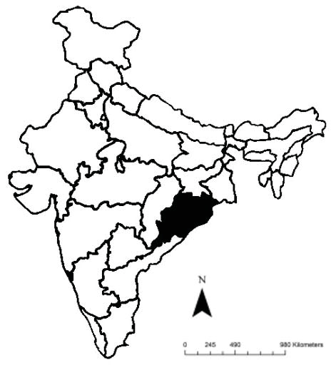
Furthermore, Odisha’s location (extending from 17.31-22.31N latitude and 81.31-87.29E longitude) in the tropical zone makes it susceptible to high temperatures and humidity fluctuations. For instance, in recent decades, Odisha has frequently faced weather extremes, such as droughts, floods, storms, tropical cyclones and more (Srinivasa Rao et al., 2016). A limited number of studies in the literature have evaluated the impact of weather variations on the farm production and productivity of Odisha agriculture (Hoda et al., 2021; Senapati, 2022). However, the effects of weather variations on land use are yet to be examined. Hence, the paper discusses the dynamic effects of weather variations on crop yields, land use and intensity in eastern India, setting it apart from traditional studies that primarily focus on the impact of climate on yields. The study uses the panel auto-regressive distributed lag (P-ARDL) method using district-level data2 for 2001-2018, with 540 total observations. Land use is the ratio of land used for agriculture to non-agricultural uses. Finally, variables like crop diversification represent land use patterns, and cropping intensity represents land use intensity. The results underscore the significance of dynamic effects, revealing patterns and insights that static analyses would miss.
This study makes several significant contributions to the literature. First, it enhances our understanding of how land use patterns and intensity respond to long-term changes in precipitation and temperature, which is crucial for improving crop yields, productivity, food security and livelihood strategies in India and other developing and emerging economies. Second, the findings can assist policymakers in formulating incentives to encourage future adaptation strategies in response to increasing weather risks. Third, the study employs both short-term and long-term assessments, providing a sophisticated methodological approach. This helps in designing appropriate coping mechanisms to address the adverse impacts of weather variability and limited land. Finally, the findings are applicable to various other states in India, including West Bengal, Bihar, Assam and Andhra Pradesh, which share similar agro-weather zones and agricultural practices.
The rest of the paper is organised as follows: Section 2 reviews the literature, providing the background and context for the study; Section 3 describes the data sources and methodology used in the research, detailing the analytical techniques employed; Section 4 discusses the study’s findings, interpreting the results and their implications; Section 5 concludes the paper, summarising the key insights and suggesting policy implications based on the findings.
The impact of weather variations is assessed by the effects of weather factors, like precipitation and temperature, on crop yields, and the magnitude of these effects is contingent upon the degree of change in these variables. Over the years, climate variability has influenced crop production in high-yield and high-technology agricultural areas, particularly in agriculturally based economies in developing countries (Lemi and Hailu, 2019). The impact of climate change on crop yields was different across crops in Thailand. Climate change negatively affected longan yield, whereas it positively affected maize and had no significant effect on rice yield. There was no effect of rainfall on crop yields (Kyaw et al., 2023). Crop yields are highly sensitive to temperature globally, whereas their extent varies in continents (Liu et al., 2020).
Furthermore, the combination of reduced precipitation and elevated temperatures has the potential to result in an escalation of global food prices. To mitigate this issue, farmers must use adaptive strategies to withstand the impacts of weather variations (Tuihedur Rahman et al., 2018). Studies found that compared with rainfall deficit, excess temperature negatively affects agricultural productivity more (Taraz, 2018; Zampieri et al., 2018). Tesfaye and Tirivayi (2020) noted a maximum temperature increase in the pre-monsoon period (i.e., April-June). Pattanayak and Kumar (2021) have estimated that agricultural productivity has reduced by 4.5% with a 1°C increase in temperature in India. In addition, they predicted the total factor productivity in agriculture would decline across all states by 2050. Moulkar and Peddi (2023) state that the effects of weather variables on crop yield vary in seasons and across crops. Generally, the monsoon and winter crop yields are more sensitive to temperature (minimum and maximum) and rainfall. Vogel et al. (2019) found that variation in crop yield is associated with temperature-related extremes. Climate change has threatened agricultural production in food-insecure regions of Asian countries (Habib-ur-Rahman et al., 2022).
In India, the growing threat of climate change – manifested through rising greenhouse gas emissions, erratic weather patterns, and increasing temperature anomalies – poses serious challenges to agricultural sustainability. The IPCC (2007) has underscored the long-term risks of continued fossil fuel reliance, projecting a global temperature rise of up to 6.4°C and a sea level increase of 59 cm by the century’s end if current trends persist. Empirical evidence demonstrates a strong nexus between economic growth, energy use, and emissions: a 1% increase in fossil fuel consumption and GDP can raise CO₂ emissions by 0.67% and 0.61%, respectively, while a corresponding rise in renewable energy use and agricultural productivity reduces emissions by 3.65% and 0.41% (Raihan and Tuspekova, 2022). Both long-run and short-run relationships exist between agricultural production, economic growth, and CO₂ emissions (Ali et al., 2019). Greenhouse gas emissions tend to rise with the intensification of agriculture and allied activities but can be mitigated through increased forest cover (Ahmed et al., 2025). In the Indian context, agricultural expansion and intensification are also linked to rising emissions. A study from Bangladesh shows that a 1% increase in agricultural land, crop output, and allied activities contribute to emissions growth of 0.25%, 0.29%, and 0.40%, respectively (Raihan et al., 2023). Since Bangladesh is nearer to Odisha and other states in Eastern India, the results are more relevant to the present study context.
The implications of this growth–energy–agriculture–climate nexus are particularly acute in India’s agrarian economy, where rainfall-dependent farming remains dominant. Weather variability – particularly deviations in rainfall and evapotranspiration – has directly undermined crop yields, including key staples and pulses such as groundnut and chickpea. Despite being one of the most climate-sensitive sectors, agriculture continues to receive limited policy and investment attention (Belford et al., 2022). Climate-induced weather extremes, including droughts and heatwaves, disrupt food production, inflate prices, and depress consumption, ultimately worsening household welfare, especially among smallholders and marginal farmers (Alvi et al., 2021). In Sweden, such extremes cause major yield losses (Sjulgård et al., 2023). In India, rainfall and evapotranspiration negatively affect groundnut and chickpea yields.
Methodologically, studies assessing the agricultural impacts of climate variability in India employ two dominant approaches: general equilibrium and partial equilibrium models. While general equilibrium models offer system-wide analysis, their application is limited in developing contexts due to data and specification issues (Deressa, 2007). The partial equilibrium framework – particularly econometric models such as the Ricardian approach and crop simulation models – is more prevalent. The Ricardian model, grounded in Ricardo’s (1817) theory of land rents and later adapted by Mendelsohn et al. (1994), estimates the net impact of climate variables on farmland values or productivity. It remains a widely used tool for assessing the welfare effects of climate change, though its application in India often requires careful calibration to account for heterogeneity in climate zones, cropping systems, and socio-economic conditions (Paltasingh and Goyari, 2015; Hashida and Lewis, 2022).
To address these challenges, India must adopt integrated climate adaptation strategies. These include educating farmers on climate risks, promoting diversified and resilient cropping patterns, strengthening agricultural markets, and improving access to weather forecasts and financial safety nets. As Tripathi and Mishra (2017) argue, effective adaptation requires locally contextualised measures grounded in an understanding of regional weather variability and its interaction with socio-economic drivers.
While existing literature predominantly addresses the climate impact on yields, this paper uniquely explores the dynamic effects of weather variation on crop yields, land utilisation patterns and intensity in eastern India. This study employs a P-ARDL model on micro-level data, a methodological innovation compared to previous studies. The chosen methodology allows for an in-depth analysis of dynamic effects, providing insights that static models fail to capture. First, the P-ARDL model is particularly well-suited for datasets where variables exhibit a mixed order of integration, i.e., a combination of the I(0) and I(1) series (Pesaran and Shin, 1998). This flexibility aligns with the nature of our data, as confirmed by the panel unit root tests. In contrast, dynamic panel data models (e.g., Arellano-Bond GMM) and panel cointegration techniques often require all series to be integrated in the same order, typically I(1), which was not the case in our study. Second, the P-ARDL framework allows for variable-specific lag structures, enabling us to more accurately capture the dynamic relationships among variables with differing temporal responses. Conversely, models such as dynamic fixed effects or traditional panel cointegration models generally impose uniform lag lengths across variables, which may lead to model misspecification when applied to heterogeneous datasets like ours. Third, the P-ARDL model provides a clear and tractable single-equation framework that simultaneously estimates both short-run dynamics and long-run equilibrium relationships (Pesaran et al., 1999). This dual capability simplifies interpretation and policy relevance. In contrast, cointegration-based models (e.g., Pedroni, Kao, Westerlund tests) and system-based approaches often involve more complex estimations, with increased computational burden and interpretation challenges, especially in applied settings. Last, P-ARDL is well-suited for panels with a moderate time dimension and limited cross-sections, such as ours (T = 18 years; N = 30 districts), and performs robustly in small samples. In contrast, GMM-based dynamic panel data models can suffer from finite-sample bias and over-identification problems, especially when the number of instruments exceeds the number of cross-sectional units.
3.1 Data sources and variable construction
The study uses data from 30 districts of Odisha (see Figure 1) from 2001 to 2018 from various secondary sources such as the Department of Agriculture and Farmers’ Empowerment (Odisha Agriculture Statistics 2001-18), ENVIS Centre of Odisha’s State of Environment and the Crop Production Statistics Information System (CPSIS).
This study uses specific data on the area, production and yield of nine major crops – rice, wheat, maize, horse gram, green gram, black gram, groundnut, rapeseed and sesamum – these crops are among the major seasonal crops produced in Odisha, India3. Furthermore, the study uses other control variables, such as fertiliser consumption and agricultural credit, along with a group of weather factors, such as rainfall and maximum and minimum temperatures. We use the rainfall deviation from the normal rainfall ( ) instead of rainfall itself. The expression is standardised as , where is the standard deviation of rainfall (see Table 1 for variable description).
Data on weather factors related to the Monsoon cropping season are collected from secondary sources, comprising different phenological stages of crop growth, such as sowing and growing. The crop yield of all major crops is taken as the dependent variable in different crop yield response models. The study uses three definitions of agricultural land use patterns: (1) cropping intensity, (2) crop diversification, and (3) ratio of land use to non-farm land use pattern. Cropping intensity is the ratio of gross cropped area to net sown area as , where GCA is the gross cropped area, and NSA is the net sown area in Odisha’s agriculture, which measures how intensively the land is used for farming purposes.
The second definition is crop diversification. Crop diversification is a measure that indicates the degree of diverse patterns of land use in a farming system. Usually, farmers adopt crop diversification as a traditional strategy to minimise weather risks. This helps stabilise farm income volatility and augments income levels (Basantaray et al., 2022). It also helps retain and revive soil health. Several diversification measures are available in the literature, but we use the Composite Entropy Index4, defined as: where CEI has two components: distribution and number of crops (N) or diversity. Here is the share of th crop in total operational landholding.
The value of the CEI increases with the rise in the number of crops and decreases in concentration. The value of CEI ranges between zero and one, indicating no diversification to perfect diversification. The third variable that captures the land use rate is the rate of agricultural use of land, which is defined again as the ratio of total cultivable (000’ ha) land under agricultural use to non-agricultural use and is formally expressed as where ALU stands for the rate of agricultural use of land, is the total land under agricultural use, and LNAt is the total land under non-agricultural use. This measure gives us a broad idea of how the cultivable landmass is used for farming purposes and the trend over time. All these variables are gathered annually, and the total observations are 540. All variables and their definitions are described in Table A1.
3.2 Empirical estimation methods
To prepare for the panel ARDL estimation, we first conduct descriptive statistics and correlation analysis to examine the central tendencies, dispersion, and pairwise relationships among the study variables – namely, crop yield, land use, rainfall deviation, and temperature variation. To assess the stationarity of these variables, we apply panel unit root tests, including the Levin-Lin-Chu (LLC) test (Levin et al., 2002) and the Im-Pesaran-Shin (IPS) test (Im et al., 2003), both of which are extensions of the augmented Dickey-Fuller (ADF) test and assume cross-sectional independence. The P-ARDL model is suitable when the panel data series are either I(0), I(1), or a combination of both, but not I(2). If any variable is found to be integrated with order two (I(2)), we exclude it from the estimation to maintain model validity. The panel ADF unit-root test estimates the following model:
(1)
where in Eq. (1), is the random process of one variable, the period t = 1, 2…, T and i = 1, 2,…,N represents the cross-sectional units/groups. If the unit-root test results show that the variables are stationary, either in I(0) or I(1) or mixed order of integration, then the P-ARDL model is applied to explore the impact of weather variations and other factors on crop yields, rate, pattern and intensity of land use. Otherwise, in the case of non-stationary or stationary in different order, either I(1) or I(2), the Todo-Yamato causality test and vector error-correction (VEC) model are appropriate to measure the effects. We estimated the following baseline model using panel ARDL to carry out our objective as we get mixed stationarity conditions of variables:
(2)
The dependent variable is estimated for all nine major crops and three different forms of land use. The other control variables, such as areas under high-yielding varieties (HYVA), total fertiliser consumption (FERT) and agricultural credit from banks (CRD), are also modelled. Although the variables are in different units, they are taken in logarithmic values to estimate the log-linear model from Eq. (2) for better analysis of results. The coefficients can be directly interpreted as elasticity values.
3.3 P-ARDL model specification
To term a P-ARDL model, we must first determine the optimal lag length. This has been done using the Schwarz information criterion (SIC), which indicates one lag as the optimum lag for use in the P-ARDL model, which estimates both long-term and short-term relationships between variables5. Moreover, the dynamic heterogeneous P-ARDL model developed by Pesaran and Shin (1998) and Pesaran et al. (1999) can be expressed within the (p,q) lag approach. The period t=1, 2…T and groups i=1, 2…N. It is expressed as:
(3)
where is the dependent variable (crop yields, cropping intensity and rate of land use), is (K×1) vector of explanatory variables. The parameter vector of the order (K×1) is the coefficient vector of the lagged dependent variable, is the vector of coefficients of all explanatory variables to be estimated, is a unit-specific fixed effect and is an error term. Both p and q are optimal lag orders.
If the variables in Eq. (3) are I(1) and cointegrated, formerly, the error term is an I(0) for all i. A salient feature of cointegrated variables is that they respond to any deviation in the long-term equilibrium relationship. This means that the deviation from the long-term equilibrium captured by the error correction model (ECM) reveals the short-term dynamics of the variables. Hence, the short-term relationship between the study variables, the error correction model (ECM), is estimated based on the framework of (p, q) as:
(4)
where
;
;
; j = 1, 2, …p-1 and
; j=1, 2, 3…q-1.
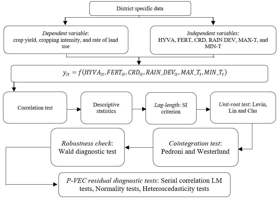
In the above Eq. (4), is the ECM coefficient for each unit, and its value indicates the adjustment rate to the long-term equilibrium. The term should be negative and significant. If then we don’t have a long-term relationship. Pesaran, Shin and Smith (1999) developed a pooled mean group (PMG) estimator that combines mean and pooling residuals, and this test incorporates the intercept, short-term coefficients and different error variances across the groups. However, based on this test, long-term coefficients are assumed to be equal across the groups, like fixed effect estimators. This P-ARDL model can be applied when variables are of the order I (0), I (1) or a mix of both. A flowchart showing related data diagnosis is presented in Figure 2. All estimations, including the P-ARDL model and diagnostic tests6, were carried out using EVIEWS-13 software.
4.1 Results of descriptive statistics
Table 1 reports the descriptive statistics of the study variables7. The results indicate that among the cereal crops, rice yield has the highest mean value (1580.30 kg/ha) and the standard deviation (589.85), followed by wheat and maize yields (1393.79 kg/ha and 1376.35 kg/ha), and wheat yield has the lowest standard deviation (521.79). The pulse crop yield indicates that horse gram yield has a higher mean value of (317.35 kg/ha) than green gram yield (297.08 kg/ha) and black gram yield (290.69 kg/ha), but horse gram has a lower standard deviation (99.10) than other pulse productions. Among the oilseeds, groundnut has a higher mean value (1145 kg/ha) and standard deviation (411.85) than rapeseed and sesamum seeds. The skewness values of all crops’ productions are negative, except for maize and rapeseed, and kurtosis values are positive, indicating negatively skewed crop production. Similarly, the crop yield statistics indicate that the mean value of rice, wheat, maize and groundnut yields are positive and other crop yields are negative. The standard deviation of maize yield is the highest (802.86 kg/ha), followed by rice yield, whereas the least standard deviation is found in horse gram (99.10). Among the weather variables, rainfall has higher mean and standard deviation values (153.15 mm and 2.10mm) than temperatures. The mean values of fertiliser consumption and agriculture land use are (320.83kg/ha and 0.26). The mean values of cropping intensity and its standard deviation values are positive. The skewness and kurtosis values are also positive and very high.
| Variables | Mean | Std. Dev. | Skewness | Kurtosis | Jarque-Bera | Probability | |||||||||||||
|---|---|---|---|---|---|---|---|---|---|---|---|---|---|---|---|---|---|---|---|
| Rice yield (RICEY) | 1580.30 | 589.85 | 0.37 | 3.15 | 13.02 | 0.00 | |||||||||||||
| Wheat yield (WHEATY) | 1393.79 | 521.79 | 0.15 | 8.18 | 606.32 | 0.00 | |||||||||||||
| Maize yield (MAIZEY) | 1376.35 | 802.86 | 2.95 | 20.12 | 7376.99 | 0.00 | |||||||||||||
| Horse gram yield (HGRAMY) | 317.80 | 99.10 | 0.86 | 6.49 | 339.92 | 0.00 | |||||||||||||
| Green gram yield (MONGY) | 297.08 | 114.94 | 1.03 | 5.23 | 207.45 | 0.00 | |||||||||||||
| Urad yield (URADY) | 290.69 | 109.84 | 0.97 | 4.99 | 174.19 | 0.00 | |||||||||||||
| Groundnut yield (GNUTY) | 1145.17 | 411.85 | 1.73 | 8.97 | 1069.40 | 0.00 | |||||||||||||
| Rapeseed yield (RPSEEDY) | 832.24 | 144.51 | 3.17 | 37.92 | 6486.00 | 0.00 | |||||||||||||
| Sesamum yield (SESAY) | 255.92 | 105.98 | 0.64 | 3.49 | 41.95 | 0.00 | |||||||||||||
| Credit (CR.) | 2.03 | 0.53 | -0.24 | 2.48 | 11.04 | 0.00 | |||||||||||||
| Fertiliser consumption (FERT) | 320.83 | 268.14 | 20.24 | 43.73 | 4615.00 | 0.00 | |||||||||||||
| Rainfall deviation (RAIN_DEV) | 153.15 | 2.10 | 0.88 | 10.89 | 1414.87 | 0.00 | |||||||||||||
| Maximum temperature (MAX_T) | 35.25 | 0.03 | -0.05 | 2.58 | 3.92 | 0.14 | |||||||||||||
| Minimum temperature (MIN_T) | 23.00 | 0.05 | -0.43 | 3.89 | 33.34 | 0.00 | |||||||||||||
| Cropping intensity (CROPINT) | 2.32 | 2.73 | 3.77 | 19.14 | 6879.20 | 0.00 | |||||||||||||
| Rate of agr. Land use (ALU) | 0.26 | 0.39 | 0.52 | 5.18 | 126.44 | 0.00 | |||||||||||||
| Crop diversification (CEI) | 0.21 | 0.11 | 0.29 | 2.19 | 21.77 | 0.00 | |||||||||||||
| Source: Authors’ calculation. Note: Initial data is parenthesis. | |||||||||||||||||||
The cross-correlations between study-selected crop yields and other variables are reported in Table A2, which indicates that all crop yields are positively influenced by their production, fertiliser consumption, agricultural credit and agricultural land use. Among the weather variables, rainfall positively correlates with crop yields, whereas the temperature correlation varies among crops. The maximum temperature negatively correlates with the crop yields, except for the wheat yield. On the other hand, the minimum temperature8 positively correlates with crop yields except for wheat and rapeseed crops. The cropping intensity is positively correlated with rice, wheat, maize and groundnut, and it is harmful to other crop yields. The Jarque-Beara test statistics and their respective probability values indicate that except for the Max_T variable, all variables are significant at a 1% significance level, which means the study variables are normally distributed.
4.2 Results of the unit-root test and VAR lag selection
Before applying the P-ARDL model, it is necessary to test the stationarity condition of variables by using unit-root tests, which will determine the reliability of the subsequent model to determine whether variables are I(0) or I(1) or a mixed order of both, but should not be I(2). The stationarity of all variables is checked using Im et al. (2003), and Levin et al. (2002), and the results are reported in Table A3. Table A3 reveals that the crop production and yields are stationary at their level values except for wheat yield, maize, horse gram and sesamum yields, and all of them are stationary at their first difference.
Other variables like fertiliser consumption, agricultural credit, weather variables like rainfall deviation and temperatures, crop diversification, cropping intensity and rate of agricultural land use are stationary at their level. We find a mixed order of stationarity of variables from the estimated unit-root test results, which suggests the suitability of the P-ARDL model. The estimation of the P-ARDL model needs an appropriate lag length. The lag selection criteria decide the optimum lag length in model estimation. Table A4 reports the results of the optimum lag selection criteria, where the SIC suggests that one is the optimum lag, the least lag among all other criteria. We use one lag, as indicated by the SIC.
4.3 Crop yield response to weather variation
Table 2 reports both the long-term relationship between the study variables and the error correction results for the short-term relations between the variables. From the long-term equation, it is found that agricultural credit significantly and positively influences all crop yields, which means if agricultural credit increases by 1%, rice yield will increase by 0.04%, wheat yield by 0.13%, horse gram yield by 0.08%, green gram (moong) yield by 0.19%, black gram yield by 0.16%, groundnut yield by 0.08%, rapeseed yield by 0.11% and sesamum seed by 0.09%. Similarly, weather variables, such as rainfall deviation and temperatures, have mixed effects on crop yields. If rainfall deviation (both excess or deficit) increases by 1%, yields of wheat decrease by 0.16%, maize by 0.46%, green gram by 0.48%, black gram by 0.06%, rapeseed by 0.28% and sesamum seed by 0.35%, but the yield of horse gram increases by 0.15%. Rainfall deviation has no significant impact on the yields of rice and groundnut. This is because rice is a water-guzzling crop, and any positive or negative deviation in rainfall affects its yield the least unless there is a large variation. Odisha agriculture is highly dominated by rice, and farmers mostly grow modern varieties that are either drought- or flood-resistant, depending on the state’s agro-weather zone. Similarly, a 1oC increase in maximum temperature significantly increases rice yield by 1.28%, maize by 0.66% and sesamum by 0.90%.
| Rice | Wheat | Maize | Horse gram | Moong | Urad | Groundnut | Rapeseed | Sesa | |||||||||||
|---|---|---|---|---|---|---|---|---|---|---|---|---|---|---|---|---|---|---|---|
| Long term Elasticities | |||||||||||||||||||
| HYVA | 0.87*** | 0.08*** | 0.11*** | 0.12*** | 0.22*** | 0.15*** | -0.03* | 0.05*** | 0.03*** | ||||||||||
| (0.02) | (0.01) | (0.03) | (0.02) | (0.03) | (0.02) | (0.02) | (0.01) | (0.01) | |||||||||||
| FERT | -0.07** | -0.06* | 0.16*** | 0.15*** | 0.07 | -0.14*** | 0.14** | -0.12*** | 0.04 | ||||||||||
| (0.04) | (0.03) | (0.04) | (0.03) | (0.06) | (0.03) | (0.05) | (0.02) | (0.04) | |||||||||||
| CRD | 0.04*** | 0.13*** | 0.01 | 0.08*** | 0.19*** | 0.16*** | 0.08*** | 0.11*** | 0.09*** | ||||||||||
| (0.01) | (0.01) | (0.02) | (0.01) | (0.02) | (0.01) | (0.01) | (0.001) | (0.01) | |||||||||||
| RAIN_DEV | -0.05 | -0.16*** | -0.46*** | 0.15*** | -0.48*** | -0.06* | 0.06 | -0.28*** | -0.35*** | ||||||||||
| (0.04) | (0.05) | (0.09) | (0.05) | (0.10) | (0.03) | (0.05) | (0.03) | (0.04) | |||||||||||
| MAX_T | 1.48*** | -0.48* | 0.66** | -0.49** | 0.40 | -1.54*** | -1.83** | -0.78** | 0.90** | ||||||||||
| (0.40) | (0.27) | (0.34) | (0.23) | (0.53) | (0.18) | (0.40) | (0.30) | (0.37) | |||||||||||
| MIN_T | 0.94*** | -0.89*** | -0.08 | 0.17 | -0.67*** | 0.61*** | 0.15 | -0.87*** | -0.48*** | ||||||||||
| (0.15) | (0.15) | (0.16) | (0.12) | (0.22) | (0.04) | (0.11) | (0.17) | (0.14) | |||||||||||
| Short term Elasticities | |||||||||||||||||||
| ECM(-1) | -0.69*** | -0.80*** | -0.33*** | -0.60*** | -0.46*** | -0.35*** | -0.46*** | -0.46*** | -0.71*** | ||||||||||
| (0.09) | (0.08) | (0.06) | (0.08) | (0.05) | (0.05) | (0.07) | (0.10) | (0.14) | |||||||||||
| ∆ (HYVA) | 0.11 | 0.02 | 0.17*** | 0.23*** | 0.15*** | 0.27*** | 0.15*** | 0.20*** | 0.16*** | ||||||||||
| (0.09) | (0.02) | (0.03) | (0.03) | (0.04) | (0.03) | (0.03) | (0.03) | (0.03) | |||||||||||
| ∆(FERT) | -0.04 | -0.11* | 0.15 | 0.04 | 0.05 | 0.05 | 0.11 | -0.03 | 0.01 | ||||||||||
| (0.08) | (0.06) | (0.11) | (0.08) | (0.06) | (0.06) | (0.09) | (0.08) | (0.13) | |||||||||||
| ∆(CR.) | -0.02 | -0.04 | -0.08 | -0.03 | 0.001 | -0.09** | -0.03 | -0.08 | -0.05 | ||||||||||
| (0.06) | (0.06) | (0.05) | (0.06) | (0.03) | (0.04) | (0.03) | (0.05) | (0.06) | |||||||||||
| ∆(RAIN_DEV) | 0.14 | 0.25*** | 0.07 | -0.04 | 0.18*** | 0.14*** | 0.15*** | 0.11 | 0.18* | ||||||||||
| (0.07) | (0.07) | (0.09) | (0.06) | (0.06) | (0.06) | (0.05) | (0.06) | (0.11) | |||||||||||
| ∆(MAX_T) | -0.67*** | -0.17*** | -0.94 | 0.5 | -1.20*** | -2.63*** | 0.86 | 0.02 | 0.81 | ||||||||||
| (0.09) | (1.27) | (1.01) | (0.37) | (0.60) | (0.74) | (0.83) | (0.83) | (0.84) | |||||||||||
| ∆(MIN_T) | 0.01 | 0.09 | 0.3 | 0.69* | -0.28 | -0.54 | 0.41 | 1.01* | -0.31 | ||||||||||
| (0.90) | (0.47) | (0.73) | (0.40) | (0.46) | (0.51) | (0.62) | (0.59) | (0.72) | |||||||||||
| Const. | -5.31*** | 1.62 | 0.27*** | -0.30*** | 0.21*** | 0.07*** | 1.27*** | 0.91 | -0.26*** | ||||||||||
| (0.73) | (0.16) | (0.05) | (0.03) | (0.03) | (0.01) | (0.20) | (0.20) | (0.05) | |||||||||||
| Source: Authors’ calculation. Note: *** P < 0.01%, ** P< 0.05% and * P < 0.10. The coefficients of lagged values of yields are not reported. Standard errors in parenthesis. | |||||||||||||||||||
On the other hand, a 1oC increase in maximum temperature leads to a decrease in the yields of wheat by 0.48%, horse gram by 0.49%, black gram by 1.54%, groundnut by 1.83% and rapeseed by 0.78%; there is no significant impact on the green gram yield. The minimum temperature increase negatively affects wheat, green gram, rapeseed and sesamum yields but positively impacts rice and black gram yields. Except for agricultural credit and weather factors, other variables, such as the area under high-yield-variety seeds and fertiliser consumption, significantly affect crop yields. It is found that the HYVA coefficients are significant and positive except for groundnut, which means if the area under high-yield-variety crops increases by 1%, the yield of rice increases by 0.87%, wheat by 0.08%, maize by 0.11%, moong by 0.22%, black gram by 0.15%, rapeseed by 0.05% and sesamum seed by 0.03%. In contrast, groundnut yield decreases by 0.03%. Similarly, suppose fertiliser consumption increases by 1%. In that case, crop yields decrease, such as rice yield decreasing by 0.07%, wheat yield decreasing by 0.06%, black gram yield decreasing by 0.14% and rapeseed yield decreasing by 12%.
The results of the short-term equation (Eq. 4) show that the ECM coefficients are significantly negative in all crop yields, indicating a need for short-term adjustment for a long-term equilibrium relationship between the study variables. The coefficient of agricultural credit is significantly negative only on the black gram yield, whereas there is no significant effect in all other crop yield models. The rainfall deviation significantly positively impacts green gram, black gram, groundnut, wheat and sesamum yields. Since these are mostly pulses and oilseeds grown in rain-fed areas, they consume less water. So, any negative deviation may not harm their yield to a great extent. However, any positive deviation may positively affect their yield because it offers the required amount of moisture rather than creating a flood-like situation. These crops are grown when the monsoon period is over. So, the positive deviation over the normal trend helps the crops rather than creating a flood-like situation and reaps better yields of these dry-area crops. The maximum temperature significantly negatively impacts rice, wheat, green gram (moong) and black gram yields.
Similarly, the minimum temperature significantly and positively affects the horse gram and rapeseed yield, but it has no significant effect on all other crops. Fertiliser consumption is significantly negative only in wheat yield. The high-yielding-variety coefficients are significant and positive for almost all crops, which indicates that if the area under high-yielding varieties increases in the short term by 1%, the yields of maize, horse gram, moong, black gram, groundnut, rapeseed and sesamum seed rise.
4.4 Land use response to weather variation
Table 3 reports the P-ARDL results of the impact of weather factors and other control variables on land use patterns and intensity. Since we have used three variables representing the rate, pattern and intensity of land use, i.e., rate of land use (ALU), crop diversification (CEI) and cropping intensity (CROPINT), we present the results separately. Here, we also have both long-term and short-term dynamics. We offer the long-term results first and then the short-term effects.
| CROPINT | ALU | CEI | |||||||||||||||||
|---|---|---|---|---|---|---|---|---|---|---|---|---|---|---|---|---|---|---|---|
| Long term elasticities | |||||||||||||||||||
| FERT | 0.08*** (0.02) |
0.53*** (0.08) |
0.07 (0.06) |
||||||||||||||||
| CRED | 0.02*** (0.01) |
0.19*** (0.02) |
0.19** (0.06) |
||||||||||||||||
| RAIN_DEV | -0.16*** (0.03) |
-0.20* (0.11) |
0.11** (0.05) |
||||||||||||||||
| MAX_T | -0.68*** (0.16) |
-1.36** (0.68) |
0.29*** (0.01) |
||||||||||||||||
| MIN_T | -0.01 (0.07) |
-1.06*** (0.29) |
0.58 (0.61) |
||||||||||||||||
| Short term elasticities | |||||||||||||||||||
| ECM (-1) | -0.52*** (0.05) |
-0.66*** (0.08) |
-61*** (0.06) |
||||||||||||||||
| ∆(CROINT (-1)) | -0.338 *** (0.044) |
||||||||||||||||||
| ∆(ALU (-1)) | -0.449*** (0.042) |
||||||||||||||||||
| ∆(CEI (-1)) | -0.584*** (0.049) |
||||||||||||||||||
| ∆(FERT) | 0.01 (0.02) |
0.16 (0.12) |
0.21* (0.12) |
||||||||||||||||
| ∆(CRD) | 0.03* (0.01) |
-0.05 (0.08) |
0.02 (0.05) |
||||||||||||||||
| ∆(RAIN_DEV) | -0.01 (0.01) |
-0.15 (0.11) |
0.88*** (0.12) |
||||||||||||||||
| ∆(MAX_T) | -0.14 (0.23) |
-2.96* (1.59) |
1.12* (0.56) |
||||||||||||||||
| ∆(MIN_T) | -0.20* (0.10) |
-0.28 (1.36) |
-0.56 (0.41) |
||||||||||||||||
| Const. | 1.53 (0.14) |
-2.28*** (0.26) |
1.47** (0.65) |
||||||||||||||||
| Source: Authors’ calculation. Note: *** P < 0.01%, ** P < 0.05% and * P < 0.10. Variables are naturally log-transformed. In case of rainfall deviation, the absolute value is taken for log transformation. Standard errors in parenthesis. | |||||||||||||||||||
We observed that rainfall deviation significantly harms cropping intensity. More specifically, its elasticity coefficient indicates an additional 1% increase in rainfall deviation, reducing the cropping intensity by 0.16%. It hampers both the gross cropped area and the net sown area. However, it affects the gross cropped area more than the net sown area, reducing the cropping intensity. This is because rainfall deviation, either upward or downward, creates a flood- or drought-like situation affecting farming practices and ultimately decreasing the gross cropped area.
On the other hand, the net sown area is somewhat determined by the irrigation potential being used. So, it reduces the numerator of the ratio more than the denominator, reducing the cropping intensity. Sometimes, delays in the arrival of monsoons also adversely affect soil preparation and sowing/planting of seedlings. This also harms farming by reducing the gross cropped area. Naturally, a delayed monsoon will have more deviations in precipitation by disturbing its spatiotemporal distribution. Our result aligns with other studies in African countries, such as those of Duku et al. (2018).
Similarly, as the negative elasticity coefficient of maximum temperature suggests, a 1% increase in maximum temperature (MAX_T) may reduce the cropping intensity (CROPINT) by 0.68% over the long term. A plausible explanation is that a rise in temperature reduces the yields of certain crops, discouraging the allotment of land to those crops (Birthal and Hazrana, 2019). Similarly, Zampieri et al. (2018) argued that excess temperatures and heatwaves affect crop yield more than drought and rainfall deviation in arid and semi-arid tropical zones. Our results are consistent with Birthal et al. (2021).
Similarly, looking into the long-term impact of weather factors on crop diversification (CEI) and rate of land use (ALU), we observe that most weather factors significantly induce crop diversification but harm the rate of land use in the long term. In fact, the elasticity coefficient of rainfall deviation concerning crop diversification shows that an additional 1% deviation in rainfall induces 0.11% more crop diversification. This is because farmers adopt diversification as an ex-ante coping mechanism to counter the production shock due to weather variations (Gouraram et al., 2022). A diversified crop portfolio helps farmers increase the resilience of their farm production system and considerably lower their exposure and vulnerability to the harmful effects of changing environmental conditions (Basantaray et al., 2022). Even in rain-fed agriculture, vertical diversification9 is adopted as an effective risk management strategy (Prasada, 2020).
Similarly, maximum temperature also positively influences crop diversification. Higher temperatures reduce soil moisture and cause dryness. So, farmers shift the cropping pattern toward pulses, which require less water and little moisture in the soil (Zampieri et al., 2018). The elasticity coefficient is 0.29, implying that an additional increase in average temperature by 1oC can induce crop diversification by 29% during the Monsoon season on a long-term basis. Moniruzzaman (2019) found similar evidence in neighbouring Bangladesh. The author simulated that increased temperature increased crop diversification over the baseline scenario of temperature and rainfall during the rainy and summer seasons.
However, rainfall deviation (RAIN_DEV) and temperature (both MAX_T and MIN_T) adversely affect the rate of land use (ALU) in the long term. As observed from the elasticity coefficient, an additional 1% increase in deviation reduces the rate of agricultural use of land by 0.20%. Rainfall deviations harm the intensity of land use and thereby affect farm production. As stressed above, any deviation from the normal level affects soil preparation and the intensive use of land for cultivation. Similarly, if the average temperatures (MAX_T and MIN_T) increase by 1oC, agricultural use of land decreases by 1.36% and 1.06%, respectively, which indicates that deviations from normal temperature levels have a severe adverse impact on the rate of agricultural use of land.
Along with weather factors, we observed that over the long term, fertiliser consumption and agricultural credit affect cropping intensity, crop diversification and rate of agricultural land use. This is because easy and smooth access to credit facilitates the investment in necessary inputs, such as seeds and other equipment, and helps prepare the soil in advance. So, this positively impacts cropping intensity and crop diversification, leading to a rise in land use.
Regarding the short-term results, we observed that all forms of land use are negatively affected by their lagged values, which is counterintuitive as per the rational expectation theory. Observing the weather factors, we find that rainfall deviation does not significantly affect cropping intensity and rate of land use in the short term, though the coefficients are intuitively negative. However, rainfall deviation does induce a substantially higher degree of diversification. The elasticity coefficient indicates that a 1% rise in rainfall deviation brings 0.88% more crop diversification. This may be attributed to the fact that a greater deviation (either positive or negative) has immediate implications for crops.
A positive deviation leads to the submergence of crops, while a shortfall of rainfall from the normal level creates a drought-like situation, leading to crop failure. In both cases, it induces more diversification as an immediate strategy in the short term to counter the crop loss caused by weather variation. Many empirical studies argue that greater agro-biodiversity contributes to increased crop yield and reduced production risk (Di Falco and Veronesi, 2014). Even farmers adopt crop diversification as an ex-ante measure to cope with weather-induced income shocks (Moniruzzaman, 2019). So, rainfall deviation has a positive impact on crop diversification. The minimum temperature significantly affects the rate of agricultural land use and crop diversification, while its elasticity coefficient in the case of cropping intensity is statistically insignificant. However, the maximum temperature adversely affects the rate of agricultural land use, while its impact on crop diversification is positive. Among other variables, we observed that credit access significantly impacts cropping intensity in the short term, while fertiliser consumption significantly induces a higher degree of crop diversification. Both elasticity coefficients are statistically significant only at a 10% probability level.
The P-ARDL model results are diagnosed using the Wald diagnostic test. This has the null hypothesis that the covariate’s coefficient is equal to zero. The Wald coefficient diagnostic test results of crop yields and land use patterns are reported in Table A5 and Table A6, which indicate that the estimated F-statistic values are highly significant, meaning that the variables are significant to the model fit. We used different model residual diagnostic tests, such as the serial correlation LM test, normality tests, and heteroscedasticity test, to check the model’s diagnostic. Table A7 presents the results of model residual diagnostic tests. All the test results indicate that all null hypotheses of all tests are statistically significant at a 1% level. That means there is a rejection of the null hypothesis concerning land use variables in all three models, which means the models are free from serial correlation and heteroscedasticity and are normally distributed.
The novelty of this study lies in considering, first, the heterogeneous impact of weather variables such as rainfall deviation and temperature, which vary among crops under study, similar to the evidence found by Guntukula and Goyari (2020). Second, rainfall deviation harms the rate and intensity of land use over both the long and short terms, but rainfall deviation induces more crop diversification. So, weather variations may distort the rate and intensity of land use, but the change in land use patterns is favourable.
The study findings have significant implications for food security and the long-term viability of the industrial system. Because almost all crop yields have been negatively damaged, predictions for food security and the sustainability of food production appear bleak. However, based on the findings, we make policy recommendations to reduce the impact of weather variations on agricultural production in the study area. Adaptive policies, strategies and weather financing must be implemented. Because temperatures and the timing and amount of necessary rainfall have changed and are expected to vary in the study region, farmers must adopt new crop types and greater diversification techniques to combat weather hazards. By highlighting dynamic effects, this study provides a more nuanced understanding of weather-induced changes in land-use intensity; the policy suggestions hover around land management and efficient use of resources. This implies developing and initiating widespread adoption of modern stress-tolerant cultivars resilient to various weather-induced stresses and making an optimal crop choice – crop diversification strategies. Such adoption should be followed by acreage allocation, considering the expected weather shocks. To help farmers, the government could invest in research and development activities to develop crop varieties resilient to extreme weather shocks.
Policymakers could provide funding for renovating the extension network to disseminate early weather warnings, thus helping sustain the optimal acreage allocation and intensity of land use. Crop diversification is an effective ex-ante coping mechanism to counter the harms induced by weather variation. However, government policy has not been conducive to a diversified production system since we somehow promote a monoculture of certain crops that the Green Revolution initiated. Odisha agriculture used to be diversified indigenously. But after the Green Revolution of the 1960s, rice has become the staple crop grown here at the expense of pulses. Though some recent concerted efforts have been made to promote crop diversification and return to indigenous cropping patterns, they have not been widely promoted. The “Millet Mission” is one such effort by the government of Odisha, but we need more such schemes that encourage diversification. We, too, found that weather variations would induce more diversification ex-post, but adopting diversification as an ex-ante strategy will be more effective. Agriculture in Odisha was traditionally characterised by a highly diversified cropping pattern. However, following the 1960s, it became increasingly concentrated around rice cultivation. A return to diversified farming systems is proposed, encouraging the cultivation of millets, pulses, and other traditional crops to restore balance and resilience in the agricultural landscape. In addition, smallholders must be covered by crop insurance and hedging as part of the formal modern weather risk-mitigating mechanism. The paper’s emphasis on dynamic effects provides a critical contribution to the field, paving the way for future studies to explore these dimensions further.
Despite the robustness of the empirical strategy and the authenticity of the data sources, this study has certain limitations. The analysis is confined to 30 districts in Odisha, which may limit the generalisability of the findings to other Indian states or agro-climatic zones. While all variables were sourced from the ENVIS Centre of Odisha’s State of Environment – an authoritative platform supported by the Ministry of Environment, Forest and Climate Change – certain critical variables such as irrigation infrastructure, mechanisation, and technological adoption were not included. These factors can influence crop yield, cropping intensity, and land use, and their omission may lead to potential biases. Moreover, the weather variables used – rainfall deviation and average temperature – do not capture the full spectrum of extreme events, intra-seasonal variability, or asymmetric effects of droughts and floods. Additionally, while the panel ARDL framework accommodates dynamic relationships, concerns related to endogeneity and omitted variables, such as input prices or market access, remain. The focus on major crops also excludes the vulnerability of minor crops and allied sectors, while the lack of socio-economic disaggregation restricts the insights for targeted policy interventions.
These limitations offer avenues for future research. Subsequent studies could incorporate more granular weather data, such as temperature thresholds, rainfall timing, or extreme weather indices, alongside farm-level primary data to better capture farmer behaviour and adaptation responses. Expanding the spatial scope to include other states with similar agro-ecological characteristics would enhance the external validity of the results. Furthermore, integrating irrigation access, mechanisation levels, crop insurance coverage, and institutional support would provide a more comprehensive understanding of the drivers of land use decisions and crop productivity under climate stress. The proposed model could also be assessed for its effectiveness in medium-term out-of-sample forecasting using approaches such as the Auto-Regressive Integrated Moving Average with exogenous variables (ARIMAX) model (Kozicka et al., 2018; Mantziaris et al., 2024) offering insights into yield responses under future weather variability, which would be of interest to both policymakers and potential investors. Future research could also explore gender- and caste-based vulnerability to weather shocks, assess the role of policy instruments such as PM-KISAN or the Millet Mission, and apply structural models or simulations to evaluate the effectiveness of proposed adaptation strategies. Taken together, the integrated approach provides valuable insights that can inform future agricultural adaptation strategies in weather-sensitive regions, thereby enriching the empirical base for designing climate-resilient agricultural policies.
This paper was presented at the Odisha Research Conclave, organised at Ravenshaw University, Cuttack, in 2023. The authors are grateful to the participants for their valuable feedback. Special thanks are extended to Amarendra Das (NISER Bhubaneswar) for his insightful suggestions. The authors also acknowledge the handling editor and anonymous reviewers of the journal for their constructive comments, which have substantially improved the quality and clarity of this paper. Any remaining errors are the sole responsibility of the authors.
The authors gratefully acknowledge the financial support provided by the Higher Education Department, Government of Odisha, India.
Ahmed, N., Xinagyu, G., Alnafissa, M., Ali, A., and Ullah, H. (2025). Linear and non-linear impact of key agricultural components on greenhouse gas emissions. Scientific Reports, 15(1): 5314. https://doi.org/10.1038/s41598-025-88159-1
Ali, S., Ying, L., Shah, T., Tariq, A., Ali Chandio, A., and Ali, I. (2019). Analysis of the Nexus of CO2 Emissions, Economic Growth, Land under Cereal Crops and Agriculture Value-Added in Pakistan Using an ARDL Approach. Energies, 12(23): 4590. https://doi.org/10.3390/en12234590
Alvi, S., Roson, R., Sartori, M., and Jamil, F. (2021). An integrated assessment model for food security under climate change for South Asia. Heliyon, 7(4): e06707 https://doi.org/10.1016/j.heliyon.2021.e06707
Arora, N. K. (2019). Impact of climate change on agriculture production and its sustainable solutions. Environmental Sustainability, 2(2): 95–96. https://doi.org/10.1007/s42398-019-00078-w
Asogwa, J., Manasseh, C., Abada, F., Nwonye, G., Nwonye, N., Okanya, O., … Okoh, J. (2022). Effect of Climate Variability on Crop Production: Evidence from Selected Communities in Rivers State Nigeria. Journal of Xi’an Shiyou University, 18(3): 239–260. https://www.xisdxjxsu.asia/viewarticle.php?aid=781
Barik, S. (2023). Odisha produces 13.606 million tonnes of food grains, highest production so far for state. The Hindu. https://www.thehindu.com/news/national/other-states/odisha-produces-13606-million-tonnes-of-food-grains-highest-production-so-far-for-state/article66899856.ece
Basantaray, A. K., Paltasingh, K. R., and Birthal, P. S. (2022). Crop Diversification, Agricultural Transition and Farm Income Growth: Evidence from Eastern India. Italian Review of Agricultural Economics (REA), 77(3): 55–65. https://doi.org/10.36253/rea-13796
Belcaid, K., and El Ghini, A. (2020). Measuring the Weather Variability Effects on the Agricultural Sector in Morocco. In J. Xu, S. E. Ahmed, F. L. Cooke, and G. Duca (Eds.), Proceedings of the Thirteenth International Conference on Management Science and Engineering Management (pp. 70–84). Cham. Springer International Publishing. https://doi.org/10.1007/978-3-030-21248-3_6
Belford, C., Huang, D., Ahmed, Y. N., Ceesay, E., and Sanyang, L. (2022). An economic assessment of the impact of climate change on the Gambia’s agriculture sector: A CGE approach. International Journal of Climate Change Strategies and Management, 15(3): 322–352. https://doi.org/10.1108/IJCCSM-01-2022-0003
Birthal, P. S., and Hazrana, J. (2019). Crop diversification and resilience of agriculture to climatic shocks: Evidence from India. Agricultural Systems, 173: 345–354. https://doi.org/10.1016/j.agsy.2019.03.005
Birthal, P. S., Hazrana, J., Negi, D. S., and Bhan, S. C. (2021). Climate change and land-use in Indian agriculture. Land Use Policy, 109: 105652. https://doi.org/10.1016/j.landusepol.2021.105652
Chandio, A. A., Jiang, Y., Rehman, A., and Rauf, A. (2020). Short and long-run impacts of climate change on agriculture: An empirical evidence from China. International Journal of Climate Change Strategies and Management, 12(2): 201–221. https://doi.org/10.1108/IJCCSM-05-2019-0026
Crofils, C., Gallic, E., and Vermandel, G. (2025). The dynamic effects of weather shocks on agricultural production. Journal of Environmental Economics and Management, 130: 103078. https://doi.org/10.1016/j.jeem.2024.103078
Deressa, T. T. (2007). Measuring the economic impact of climate change on Ethiopian agriculture: Ricardian approach (Working Paper Series No. 4342). Washington D.C. The World Bank. http://documents.worldbank.org/curated/en/143291468035673156/Measuring-the-economic-impact-of-climate-change-on-Ethiopian-agriculture-Ricardian-approach
Di Falco, S., and Veronesi, M. (2014). Managing Environmental Risk in Presence of Climate Change: The Role of Adaptation in the Nile Basin of Ethiopia. Environmental and Resource Economics, 57(4): 553–577. https://doi.org/10.1007/s10640-013-9696-1
Dudu, H., and Çakmak, E. H. (2018). Climate change and agriculture: An integrated approach to evaluate economy-wide effects for Turkey. Climate and Development, 10(3): 275–288. https://doi.org/10.1080/17565529.2017.1372259
Duku, C., Zwart, S. J., and Hein, L. (2018). Impacts of climate change on cropping patterns in a tropical, sub-humid watershed. PLOS ONE, 13(3): e0192642. https://doi.org/10.1371/journal.pone.0192642
GOO. (2022). Odisha Economic Survey 2021-22. Cuttack. Directorate of Economics and Statistics Planning and Convergence Department, Government of Odisha. https://finance.odisha.gov.in/sites/default/files/2022-03/Economic%20Survey%20-%20Highlights.pdf
Gouraram, P., Goyari, P., and Paltasingh, K. R. (2022). Rice ecosystem heterogeneity and determinants of climate risk adaptation in Indian agriculture: Farm-level evidence. Journal of Agribusiness in Developing and Emerging Economies, 14(2): 146–160. https://doi.org/10.1108/JADEE-03-2022-0044
Guntukula, R., and Goyari, P. (2020). Climate Change Effects on the Crop Yield and Its Variability in Telangana, India. Studies in Microeconomics, 8(1): 119–148. https://doi.org/10.1177/2321022220923197
Habib-ur-Rahman, M., Ahmad, A., Raza, A., Hasnain, M. U., Alharby, H. F., Alzahrani, Y. M., … EL Sabagh, A. (2022). Impact of climate change on agricultural production; Issues, challenges, and opportunities in Asia. Frontiers in Plant Science, 13. https://doi.org/10.3389/fpls.2022.925548
Hashida, Y., and Lewis, D. J. (2022). Estimating welfare impacts of climate change using a discrete-choice model of land management: An application to western U.S. forestry. Resource and Energy Economics, 68: 101295. https://doi.org/10.1016/j.reseneeco.2022.101295
Hoda, A., Gulati, A., Wardhan, H., and Rajkhowa, P. (2021). Drivers of Agricultural Growth in Odisha. In A. Gulati, R. Roy, and S. Saini (Eds.), Revitalizing Indian Agriculture and Boosting Farmer Incomes (pp. 247–278). Singapore. Springer Nature. https://doi.org/10.1007/978-981-15-9335-2_9
Im, K. S., Pesaran, M. H., and Shin, Y. (2003). Testing for unit roots in heterogeneous panels. Journal of Econometrics, 115(1): 53–74. https://doi.org/10.1016/S0304-4076(03)00092-7
IPCC. (2007). Climate Change 2007: Impacts, Adaptation and Vulnerability. Geneva. Intergovernmental Panel on Climate Change. https://www.ipcc.ch/report/ar4/wg2/
IPCC. (2014). Point of Departure. In Climate Change 2014 – Impacts, Adaptation and Vulnerability: Part A: Global and Sectoral Aspects: Working Group II Contribution to the IPCC Fifth Assessment Report: Volume 1: Global and Sectoral Aspects (Vol. 1, pp. 169–194). Cambridge. Cambridge University Press. https://doi.org/10.1017/CBO9781107415379.006
Kozicka, M., Tacconi, F., Horna, D., and Gotor, E. (2018). Forecasting cocoa yields for 2050 (p. 49). Rome. Bioversity International. https://hdl.handle.net/10568/93236
Kyaw, Y., Nguyen, T. P. L., Winijkul, E., Xue, W., and Virdis, S. G. P. (2023). The Effect of Climate Variability on Cultivated Crops’ Yield and Farm Income in Chiang Mai Province, Thailand. Climate, 11(10): 204. https://doi.org/10.3390/cli11100204
Lemi, T., and Hailu, F. (2019). Effects of Climate Change Variability on Agricultural Productivity. International Journal of Environmental Sciences & Natural Resources, 17(1): 1–7. https://doi.org/10.19080/IJESNR.2019.17.555953
Levin, A., Lin, C.-F., and James Chu, C.-S. (2002). Unit root tests in panel data: Asymptotic and finite-sample properties. Journal of Econometrics, 108(1): 1–24. https://doi.org/10.1016/S0304-4076(01)00098-7
Lin, S.-S., Zhang, N., Xu, Y.-S., and Hino, T. (2020). Lesson Learned from Catastrophic Floods in Western Japan in 2018: Sustainable Perspective Analysis. Water, 12(9): 2489. https://doi.org/10.3390/w12092489
Liu, D., Mishra, A. K., and Ray, D. K. (2020). Sensitivity of global major crop yields to climate variables: A non-parametric elasticity analysis. Science of The Total Environment, 748: 141431. https://doi.org/10.1016/j.scitotenv.2020.141431
Mantziaris, S., Rozakis, S., Karanikolas, P., Petsakos, A., and Tsiboukas, K. (2024). Simulating farm structural change dynamics in Thessaly (Greece) using a recursive programming model. Bio-Based and Applied Economics, 13(4): 353–386. https://doi.org/10.36253/bae-14790
Martin-Moreno, J. M., Garcia-Lopez, E., Guerrero-Fernandez, M., Alfonso-Sanchez, J. L., and Barach, P. (2025). Devastating “DANA” Floods in Valencia: Insights on Resilience, Challenges, and Strategies Addressing Future Disasters. Public Health Reviews, 46: 1608297. https://doi.org/10.3389/phrs.2025.1608297
Mendelsohn, R., Nordhaus, W. D., and Shaw, D. (1994). The Impact of Global Warming on Agriculture: A Ricardian Analysis. The American Economic Review, 84(4): 753–771. https://www.jstor.org/stable/2118029
Mohapatra, S., Paltasingh, K. R., Peddi, D., Sahoo, D., Sahoo, A. K., and Mohanty, P. (2025). Evaluating Seasonal Weather Risks on Cereal Yield Distributions in Southern India. Journal of Quantitative Economics. https://doi.org/10.1007/s40953-025-00448-8
Mohapatra, S., Sharp, B., Sahoo, A. K., and Sahoo, D. (2023). Seasonal Weather Sensitivity of Staple Crop Rice in South India. In P. S. Duque de Brito, J. R. da Costa Sanches Galvão, P. Monteiro, R. Panizio, L. Calado, A. C. Assis, … V. S. Santos Ribeiro (Eds.), Proceedings of the 2nd International Conference on Water Energy Food and Sustainability (ICoWEFS 2022) (pp. 130–146). Cham. Springer International Publishing. https://doi.org/10.1007/978-3-031-26849-6_15
Moniruzzaman, S. (2019). Crop diversification as climate change adaptation: How do bangladeshi farmers perform? Climate Change Economics, 10(02): 1950007. https://doi.org/10.1142/S2010007819500076
Moulkar, R., and Peddi, D. (2023). Climate sensitivity of major crops yield in Telangana state, India. Journal of the Asia Pacific Economy, 29(4): 2023–2040. https://doi.org/10.1080/13547860.2023.2230007
Nugroho, A. D., Prasada, I. Y., and Lakner, Z. (2023). Comparing the effect of climate change on agricultural competitiveness in developing and developed countries. Journal of Cleaner Production, 406: 137139. https://doi.org/10.1016/j.jclepro.2023.137139
Opoku Mensah, S., Akanpabadai, T. A., Diko, S. K., Okyere, S. A., and Benamba, C. (2023). Prioritisation of climate change adaptation strategies by smallholder farmers in semi-arid savannah agro-ecological zones: Insights from the Talensi District, Ghana. Journal of Social and Economic Development, 25(1): 232–258. https://doi.org/10.1007/s40847-022-00208-x
Paltasingh, K. R., and Goyari, P. (2015). Climatic Risks and Household Vulnerability Assessment: A Case of Paddy Growers in Odisha. Agricultural Economics Research Review, 28: 199–210. https://doi.org/10.5958/0974-0279.2015.00035.X
Pattanayak, A., and Kumar, K. S. K. (2021). Does weather sensitivity of rice yield vary across sub-regions of a country? Evidence from Eastern and Southern India. Journal of the Asia Pacific Economy, 26(1): 51–72. https://doi.org/10.1080/13547860.2020.1717300
Pattanayak, A., Kumar, K. S. K., and Anneboina, L. R. (2021). Distributional impacts of climate change on agricultural total factor productivity in India. Journal of the Asia Pacific Economy, 26(2): 381–401. https://doi.org/10.1080/13547860.2021.1917094
Pesaran, H. H., and Shin, Y. (1998). Generalised impulse response analysis in linear multivariate models. Economics Letters, 58(1): 17–29. https://doi.org/10.1016/S0165-1765(97)00214-0
Pesaran, M. H., Shin, Y., and Smith, R. P. (1999). Pooled Mean Group Estimation of Dynamic Heterogeneous Panels. Journal of the American Statistical Association, 94(446): 621–634. https://doi.org/10.2307/2670182
Prasada, D. V. P. (2020). Climate resilience and varietal choice: A path analytic model for rice in Bangladesh. Journal of Agribusiness in Developing and Emerging Economies, 12(1): 40–55. https://doi.org/10.1108/JADEE-09-2019-0135
Raihan, A., Muhtasim, D. A., Farhana, S., Hasan, M. A. U., Pavel, M. I., Faruk, O., … Mahmood, A. (2023). An econometric analysis of Greenhouse gas emissions from different agricultural factors in Bangladesh. Energy Nexus, 9: 100179. https://doi.org/10.1016/j.nexus.2023.100179
Raihan, A., and Tuspekova, A. (2022). Nexus between economic growth, energy use, agricultural productivity, and carbon dioxide emissions: New evidence from Nepal. Energy Nexus, 7: 100113. https://doi.org/10.1016/j.nexus.2022.100113
Ricardo, D. (1817). On the Principles of Political Economy, and Taxation. Cambridge. Cambridge University Press. https://doi.org/10.1017/CBO9781107589421
Rout, H. K. (2021, November 27). 30 per cent of Odisha population is poor: Niti Aayog report. The New Indian Express. https://www.newindianexpress.com/states/odisha/2021/Nov/27/30-per-centof-odisha-population-is-poor-niti-aayog-report-2388739.html
Senapati, A. K. (2022). Weather effects and their long-term impact on agricultural yields in Odisha, East India: Agricultural policy implications using NARDL approach. Journal of Public Affairs, 22(3): e2498. https://doi.org/10.1002/pa.2498
Seven, U., and Tumen, S. (2020). Agricultural Credits and Agricultural Productivity: Cross-Country Evidence (IZA Discussion Paper No. 12930). Bonn. Institute for the Study of Labor. https://doi.org/10.2139/ssrn.3534478
Siotra, V., and Kumari, S. (2024). Assessing spatiotemporal patterns of crop combination and crop concentration in Jammu Division of Jammu and Kashmir. Journal of Social and Economic Development, 27: 139-166. https://doi.org/10.1007/s40847-024-00337-5
Sjulgård, H., Keller, T., Garland, G., and Colombi, T. (2023). Relationships between weather and yield anomalies vary with crop type and latitude in Sweden. Agricultural Systems, 211: 103757. https://doi.org/10.1016/j.agsy.2023.103757
Srinivasa Rao, Ch., Gopinath, K. A., Prasad, J. V. N. S., Prasannakumar, and Singh, A. K. (2016). Chapter Four - Climate Resilient Villages for Sustainable Food Security in Tropical India: Concept, Process, Technologies, Institutions, and Impacts. In D. L. Sparks (Ed.), Advances in Agronomy (Vol. 140, pp. 101–214). Academic Press. https://doi.org/10.1016/bs.agron.2016.06.003
Taraz, V. (2018). Can farmers adapt to higher temperatures? Evidence from India. World Development, 112: 205–219. https://doi.org/10.1016/j.worlddev.2018.08.006
Tesfaye, W., and Tirivayi, N. (2020). Crop diversity, household welfare and consumption smoothing under risk: Evidence from rural Uganda. World Development, 125: 104686. https://doi.org/10.1016/j.worlddev.2019.104686
Tripathi, A., and Mishra, A. K. (2017). Knowledge and passive adaptation to climate change: An example from Indian farmers. Climate Risk Management, 16: 195–207. https://doi.org/10.1016/j.crm.2016.11.002
Tuihedur Rahman, H. M., Hickey, G. M., Ford, J. D., and Egan, M. A. (2018). Climate change research in Bangladesh: Research gaps and implications for adaptation-related decision-making. Regional Environmental Change, 18(5): 1535–1553. https://doi.org/10.1007/s10113-017-1271-9
Vogel, E., Donat, M. G., Alexander, L. V., Meinshausen, M., Ray, D. K., Karoly, D., … Frieler, K. (2019). The effects of climate extremes on global agricultural yields. Environmental Research Letters, 14(5): 054010. https://doi.org/10.1088/1748-9326/ab154b
Xiang, T., Malik, T. H., Hou, J. W., and Ma, J. (2022). The Impact of Climate Change on Agricultural Total Factor Productivity: A Cross-Country Panel Data Analysis, 1961–2013. Agriculture, 12(12): 2123. https://doi.org/10.3390/agriculture12122123
Xie, B., Brewer, M. B., Hayes, B. K., McDonald, R. I., and Newell, B. R. (2019). Predicting climate change risk perception and willingness to act. Journal of Environmental Psychology, 65: 101331. https://doi.org/10.1016/j.jenvp.2019.101331
Yamamoto, H., and Naka, T. (2021). Quantitative Analysis of the Impact of Floods on Firms’ Financial Conditions (Working Paper No. 21-E-10). Bank of Japan. https://www.boj.or.jp/en/research/wps_rev/wps_2021/wp21e10.htm
Yang, H., Cao, Y., Shi, Y., Wu, Y., Guo, W., Fu, H., and Li, Y. (2022). The Dynamic Impacts of Weather Changes on Vegetable Price Fluctuations in Shandong Province, China: An Analysis Based on VAR and TVP-VAR Models. Agronomy, 12(11): 2680. https://doi.org/10.3390/agronomy12112680
Yoshida, S., Kashima, S., Okazaki, Y., and Matsumoto, M. (2023). Effects of 2018 Japan floods on healthcare costs and service utilisation in Japan: A retrospective cohort study. BMC Public Health, 23(1): 1–10. https://doi.org/10.1186/s12889-023-15205-w
Zampieri, M., Ceglar, A., Dentener, F., and Toreti, A. (2018). Understanding and reproducing regional diversity of climate impacts on wheat yields: Current approaches, challenges and data driven limitations. Environmental Research Letters, 13(2): 021001. https://doi.org/10.1088/1748-9326/aaa00d
| Variables | Definitions | Hypothetical sign | |||||||||||||||||
|---|---|---|---|---|---|---|---|---|---|---|---|---|---|---|---|---|---|---|---|
| Dependent variable | |||||||||||||||||||
| YLD | Crop yield (kg/hectare) | ||||||||||||||||||
| CI | Cropping intensity is defined as the ratio of gross cropped area to net sown area (Index) | ||||||||||||||||||
| CEI | Crop diversification is measured by the composite entropy index | ||||||||||||||||||
| ALU | Rate of agricultural land use is defined as the ratio of land used for agriculture to non-agricultural use (Index) | ||||||||||||||||||
| Independent variables | |||||||||||||||||||
| FERT | Total fertiliser consumption (kg/ha) | + | |||||||||||||||||
| HYVA | Area under HYV or modern variety seeds (000’ acres) | + | |||||||||||||||||
| CRD | Agricultural credit from banks (Rs. billion) | + | |||||||||||||||||
| RAIN_DEV | Standardised deviation of average rainfall during the Kharif season (millimetres) from its historical normal value | +/- | |||||||||||||||||
| MAX_T | Average maximum temperature during Kharif season (Celsius) | - | |||||||||||||||||
| MIN_T | Average minimum temperature during Kharif season (Celsius) | - | |||||||||||||||||
| Source: Authors’ annotation. Note: Complied from ENVIS Centre of Odisha’s State of Environment, Odisha Agriculture Statistics (various issues) and other sources. | |||||||||||||||||||
| Cereals | Pulses | Oilseeds | |||||||||||||||||
|---|---|---|---|---|---|---|---|---|---|---|---|---|---|---|---|---|---|---|---|
| Rice | Wheat | Maize | Horse gram | Moong | Urad | Groundnut | Rapeseeds | Sesamum | |||||||||||
| HYVA | 0.52 | 0.40 | 0.22 | 0.03 | 0.22 | 0.32 | 0.33 | 0.51 | 0.08 | ||||||||||
| FERT | 0.22 | 0.02 | 0.26 | 0.25 | 0.40 | 0.34 | 0.00 | 0.30 | 0.14 | ||||||||||
| CRD | 0.27 | 0.23 | 0.49 | 0.37 | 0.53 | 0.47 | 0.30 | 0.34 | 0.35 | ||||||||||
| RAIN_DEV | 0.26 | 0.01 | 0.02 | 0.12 | 0.08 | 0.13 | 0.12 | 0.09 | 0.06 | ||||||||||
| MAX_T | -0.05 | 0.00 | -0.08 | -0.05 | -0.06 | -0.04 | -0.02 | -0.05 | -0.22 | ||||||||||
| MIN_T | 0.01 | -0.06 | 0.05 | 0.01 | 0.01 | 0.07 | 0.18 | -0.12 | 0.09 | ||||||||||
| CROPINT | 0.11 | 0.03 | 0.03 | -0.19 | -0.05 | -0.14 | 0.06 | -0.15 | -0.31 | ||||||||||
| AL | 0.45 | 0.07 | 0.18 | 0.24 | 0.29 | 0.30 | 0.38 | 0.12 | 0.25 | ||||||||||
| Source: Authors’ estimation. | |||||||||||||||||||
| Levin, Lin & Chu t* | Im, Pesaran and Shin W-stat | ||||||||||||||||||
|---|---|---|---|---|---|---|---|---|---|---|---|---|---|---|---|---|---|---|---|
| Intercept | Intercept with Trend | Intercept | Intercept with Trend | ||||||||||||||||
| Level | 1st Difference | Level | 1st Difference | Level | 1st difference | Level | 1st Difference | ||||||||||||
| RiceY | -7.84*** | - | -6.49*** | - | -6.65*** | - | -5.12*** | - | |||||||||||
| RiceP | -6.36*** | - | -1.86** | - | -7.97*** | - | -5.76*** | - | |||||||||||
| WheatY | -1.09 | -8.40*** | -2.30** | - | -3.87*** | - | -5.13*** | - | |||||||||||
| WheatP | -3.91*** | - | -4.31*** | - | -3.76*** | - | -3.26*** | - | |||||||||||
| MaizeY | -2.46** | - | -1.74** | - | -1.31 | -13.75** | -3.02*** | - | |||||||||||
| MaizeP | -1.28 | -11.38*** | -1.05 | -8.99*** | -2.66*** | - | -1.66* | - | |||||||||||
| HgramY | -6.43*** | - | -6.46*** | - | -6.04*** | - | -7.21*** | - | |||||||||||
| HgramP | 0.55 | -8.64*** | -4.01*** | - | 0.3 | -13.71** | -3.42*** | - | |||||||||||
| MoongY | -3.66*** | - | -8.17*** | - | -1.18 | -18.08** | -6.41*** | - | |||||||||||
| MoongP | -5.54*** | - | -3.12*** | - | -6.69*** | - | -3.87*** | - | |||||||||||
| UradY | -3.15*** | - | -4.57*** | - | -2.43*** | - | -5.17*** | - | |||||||||||
| UradP | -4.36*** | - | -4.49*** | - | -4.46*** | - | -4.71*** | - | |||||||||||
| GnutY | -5.14*** | - | -6.96*** | - | -3.46*** | - | -4.66*** | - | |||||||||||
| GnutP | -5.14*** | - | -2.33** | - | -3.46*** | - | -0.92 | -10.14*** | |||||||||||
| RapeseedY | -3.34*** | - | -5.96*** | - | -2.21** | - | -6.19*** | - | |||||||||||
| RpseedP | -6.16*** | - | -7.27*** | - | -6.73*** | - | -7.38*** | - | |||||||||||
| SesaY | -4.58*** | - | -6.67*** | - | -6.05*** | - | -7.23*** | - | |||||||||||
| SesaP | 1.90 | -5.98*** | -0.97 | -4.07*** | 1.03 | -11.81*** | -0.96 | -10.1*** | |||||||||||
| FERT | -5.38*** | - | -1.08 | -1.93** | -2.83*** | - | -1.55* | - | |||||||||||
| CR | -5.95*** | - | -3.05*** | -0.02 | -8.68*** | 0.82 | -6.92*** | ||||||||||||
| RAIN_DEV | -4.62*** | - | -1.67 | 2.25** | -7.71*** | - | -5*** | - | |||||||||||
| MAX_T | -8.53*** | - | -6.92*** | - | -6.96*** | - | -4.76*** | - | |||||||||||
| MIN_T | -4.95*** | - | -3.46*** | - | -4.78*** | - | -1.86** | - | |||||||||||
| CROPINT | -5.85*** | - | -2.98*** | - | -4.17*** | - | 0.29 | -7.52*** | |||||||||||
| LN | -9.55*** | -10.90*** | -5.84*** | -6.87*** | |||||||||||||||
| Source: Authors’ estimation. Note: *, ** and *** denote 10%, 5% and 1% significance levels, respectively. | |||||||||||||||||||
| Rice | Wheat | Maize | Horse-gram | Green-gram | Urad | Groundnut | Rapeseeds | Sesamum | |||||||||||
|---|---|---|---|---|---|---|---|---|---|---|---|---|---|---|---|---|---|---|---|
| F-stat | 603.01*** | 87.07*** | 18.34*** | 43.51*** | 57.83*** | 183.42*** | 25.79*** | 1130.29*** | 1156.39*** | ||||||||||
| Chi-sqr | 4221.08*** | 609.50*** | 128.39*** | 304.57*** | 404.80*** | 1283.94*** | 180.50*** | 7912.02*** | 8094.75*** | ||||||||||
| Null Hypothesis: C (1) = C (2) = C (3) = C (4) = C (5) = C (6) = C (7) = 0 | |||||||||||||||||||
| C (1) | 0.87 | 0.08 | 0.11 | 0.12 | 0.22 | 0.15 | -0.03 | 0.05 | 0.44 | ||||||||||
| 0.02 | 0.01 | 0.03 | 0.02 | 0.03 | 0.02 | 0.02 | 0.01 | 0.03 | |||||||||||
| C (2) | -0.07 | -0.06 | 0.16 | 0.15 | 0.07 | -0.14 | 0.14 | -0.12 | -0.12 | ||||||||||
| 0.04 | 0.03 | 0.04 | 0.03 | 0.06 | 0.03 | 0.05 | 0.02 | 0.02 | |||||||||||
| C (3) | -0.04 | 0.13 | 0.01 | 0.08 | 0.19 | 0.16 | 0.08 | 0.11 | 0.14 | ||||||||||
| 0.01 | 0.01 | 0.02 | 0.01 | 0.02 | 0.01 | 0.01 | 0.00 | 0.01 | |||||||||||
| C (4) | 0.30 | 0.10 | 0.07 | 0.03 | -0.01 | 0.09 | 0.12 | 0.04 | 0.06 | ||||||||||
| 0.01 | 0.02 | 0.04 | 0.02 | 0.04 | 0.02 | 0.02 | 0.01 | 0.01 | |||||||||||
| C (5) | -0.05 | -0.16 | -0.46 | 0.15 | -0.48 | -0.06 | 0.06 | -0.28 | -0.29 | ||||||||||
| 0.04 | 0.05 | 0.09 | 0.05 | 0.10 | 0.03 | 0.05 | 0.03 | 0.02 | |||||||||||
| C (6) | 1.48 | -0.48 | 0.66 | -0.49 | 0.40 | -1.54 | -1.83 | -0.78 | 0.48 | ||||||||||
| 0.40 | 0.27 | 0.34 | 0.23 | 0.53 | 0.18 | 0.40 | 0.30 | 0.17 | |||||||||||
| C (7) | 0.94 | -0.89 | -0.08 | 0.17 | -0.67 | 0.61 | 0.15 | -0.87 | 0.10 | ||||||||||
| 0.15 | 0.15 | 0.16 | 0.12 | 0.22 | 0.04 | 0.11 | 0.17 | 0.05 | |||||||||||
| Source: Authors’ estimation. Note: *, **, and *** denote 10%, 5% and 1% significance levels, respectively. | |||||||||||||||||||
| CROPINT | ALU | CEI | |||||||||||||||||
|---|---|---|---|---|---|---|---|---|---|---|---|---|---|---|---|---|---|---|---|
| F-statistic | 30.17*** | 59.26 | 33.17*** | ||||||||||||||||
| Chi-square | 150.83*** | 296.28 | 165.83*** | ||||||||||||||||
| Null Hypothesis: C (1) = C (2) = C (3) = C (4) = C (5) = 0 | |||||||||||||||||||
| C (1) | 0.08 | 0.53 | 0.09 | ||||||||||||||||
| 0.02 | 0.08 | 0.01 | |||||||||||||||||
| C (2) | 0.02 | 0.19 | 0.04 | ||||||||||||||||
| 0.01 | 0.02 | 0.01 | |||||||||||||||||
| C (3) | 0.16 | 0.20 | 0.12 | ||||||||||||||||
| 0.03 | 0.11 | 0.03 | |||||||||||||||||
| C (4) | -0.68 | 1.36 | -0.61 | ||||||||||||||||
| 0.16 | 0.68 | 0.19 | |||||||||||||||||
| C (5) | -0.01 | 1.06 | -0.02 | ||||||||||||||||
| 0.07 | 0.29 | 0.09 | |||||||||||||||||
| Source: Authors’ estimation. Note: *** denotes a 1% significance level. | |||||||||||||||||||
| CROPINT | ALU | CEI | |||||||||||||||||
|---|---|---|---|---|---|---|---|---|---|---|---|---|---|---|---|---|---|---|---|
| Serial Correlation LM Tests (H0: no serial correlation at lag order h) | |||||||||||||||||||
| Lag 1 | 164.39*** | 155.64*** | 112.67*** | ||||||||||||||||
| Lag 2 | 189.35*** | 197.83*** | 129.22*** | ||||||||||||||||
| Normality Tests (Orthogonalisation: Cholesky) | |||||||||||||||||||
| Null hypothesis: residuals are multivariate normal | |||||||||||||||||||
| Skewness (Chi-sq) | 334.89*** | 399.75*** | 418.05*** | ||||||||||||||||
| Kurtosis (Chi-sq) | 11744.56*** | 15727.93*** | 8789.53*** | ||||||||||||||||
| Jarque-Bera | 12079.44*** | 16127.68*** | 9207.58*** | ||||||||||||||||
| Heteroskedasticity Tests: No Cross Terms | |||||||||||||||||||
| Chi-square statistics | 1075.67*** | 1200.50*** | 1492.41*** | ||||||||||||||||
| Source: Authors’ estimation. Note: *** denotes a 1% significance level. | |||||||||||||||||||
1 Except a recent study by Birthal et al. (2021).
2 Districts serve as the primary administrative units within Indian states. India has approximately 766 districts, each with an average population of around 1.86 million. The state of Odisha comprises 30 districts. Accordingly, our dataset includes a total of 540 observations spanning an 18-year period.
3 Cereals: Rice and wheat – the two primary food grains, forming the staple diet and occupying the largest share of cultivated land. Pulses: Green gram, black gram, and horse gram – important protein sources, particularly in rainfed and marginal areas. These legumes also contribute to soil nitrogen fixation and improve cropping system sustainability. Oilseeds: Groundnut, rapeseed, and sesamum – key oil-producing crops suited to Odisha’s agro-climatic conditions, cultivated for edible oil and as cash crops.
4 This CEI, a modified version of Shannon-Weaver index, rectifies its drawbacks and assesses both richness and evenness which makes it possible to compare crop diversity across different places (Tesfaye and Tirivayi, 2020). So, it is an improved measure of diversification.
5 This estimation can be conducted using STATA, EVIEWS, or any suitable statistical software for time series or panel data analysis. For this study, we employed EVIEWS 13. The underlying code used in the analysis is available from the corresponding author upon reasonable request.
6 In the case of omitted variable bias or endogeneity problem, the P-ARDL model has advantage as it takes care of endogeneity by selecting the optimal time lag in the model estimation. The problem of serial correlation, normality and heteroscadasticity can be performed in diagnostic tests.
8 The minimum temperature is the minimum annual average temperature. In Odisha, for that matter in India, this minimum temperature 23 °C is absolutely normal during monsoon season. The max goes to 40-42 °C here during summer and around 30-35 °C during most of time in a year.
9 Refers to the combination of multiple cropping and industrialization. Farmers invest in horticulture, agroforestry, livestock raising, the cultivation of fragrant herbs and more, as part of this type of diversification.