Interpretable Machine Learning for the German residential rental market – shedding light into model mechanics
Nuremberg Research Institute for Cooperative Studies, Nuremberg, Germany
E-mail: severin.bachmann@gmx.net
Abstract. We compare the drivers in Machine learning models and give insights into their strengths and weaknesses predicting rental prices. The study employs SHAP values to measure feature importance. The study aims to investigate linear regression, decision tree and XGBoost algorithms. The research is unique in its application of IML methods to a large dataset of over 2.4 million observations in the German rental market and its application of comparative statistics using aggregate SHAP values. Main results are the superiority of XGB and LR showing higher SHAP values overall and thus explaining its lower predictive efficacy. DT models capture intricate interactions among variables with fewer features, while XGB accommodates more variables, emphasizing its higher complexity and thus superior performance. The top ten features for DT and XGB models show significant overlap, indicating robust concordance. Specific features are identified that distinguish the models, suggesting that a more complex model, like XGB, handles dummy variables more adeptly.
Keywords: interpretable machine learning, SHAP, real estate.
JEL code: R3.
Index
2.2 Evolution of machine learning methods
2.3 Black Box and Explainable Artificial Intelligence
3.3 Interpretable models and SHAP values
4.3 Variable description and descriptive statistics
5.2 SHAP analysis – preprocessing
Precisely forecasting and understanding the drivers of real estate rent is vital for various stakeholders like landlords, renters, investors, and real estate brokers. Hedonic pricing models, particularly linear regression (LR) of ordinary least squared regression (OLS), have been traditionally used but face challenges due to the complex nature of renting markets on the one hand (Krämer et al., 2021) and OLS’s underlying assumption like linearity on the other (Malpezzi, 2003). Advanced statistical and machine learning (ML) techniques, including Artificial Neural Networks, Random Forest, and extreme gradient boosting (XGB), have gained interest in their ability to address OLS shortcomings. The advent of ML models in the field of real estate appraisal, driven by increased processing power and digitization (Breuer and Steininger, 2020; Piegeler and Bauer, 2021), offers more precise predictions than traditional OLS regressions (Valier, 2020). However, ML models are often perceived as “black boxes” posing challenges in comprehension compared to LR (Molnar, 2022; Surkov et al., 2022). To address this, interpretable machine learning (IML) methods, also known as explainable artificial intelligence (xAI), provide a solution. These methods offer both global and local level explanations, enabling a better understanding of ML models and specific predictions (Molnar, 2022).
The study aims to shed light on the drivers of German residential rental prices within LR, decision tree (DT) and XGB algorithms using the IML approach of Shapley Additive exPlanations (SHAP) values to measure features’ importance on a comprehensive level and apply the results in various comparative approaches in order to get a hand on the mechanics driving each of the models. While literature has already proven the superiority of XGB in the German real estate market (Stang et al., 2023) and Baur et al. (2023) have shown the usefulness of SHAP values in their work using a rather small data set of 30.000 observations, this paper is the first to apply the SHAP method on a truly mass appraisal dataset with over 2.4 million observations for the German rental market. To ensure computational feasibility while preserving the robustness of model interpretability, we apply a systematic data reduction approach. Starting with over 2.4 million observations, we utilize Slovin’s Formula to determine an appropriate sample size, resulting in a reduced yet representative dataset of 2,946 observations. Furthermore, Baur et al. (2023) leave it with the depiction of standard summary plots, while our paper applies a new method of aggregating SHAP values to compare groups of variables with each other and between models. Additionally, to the best of our knowledge we are the first to show the working application of necessary data reduction method of Slovin’s Formula in real estate context without losing any power of explainability in contrast to previously applies feature reduction methods.
In a first step to show that our models behave in line with literature we first imply LR as baseline. Non-linearity is introduced leading to the exploration of DT and XGB showing that XGB performs by far the best. In a second step, we apply SHAP values to each model. Their analysis tells that the LR model’s main predictor by far surpasses all other influencers while tree-based ML methods don’t show such a top “outperformer”. The results note further differences in variable impact between LR, DT, and XGB, with LR showing overall higher SHAP values. The analysis suggests that LR’s lower predictive efficacy is due to the granularity of individual influencing variables. Dummy variables have weaker predictive power in LR compared to DT and XGB. The significance of dummy variables increases with model complexity. Results show that DT captures intricate interactions among variables with fewer features, as it shows a significant number of features having an average absolute SHAP value of 0. In contrast, XGB, with superior performance, accommodates more variables, emphasizing the model’s capability of representing higher complexity. Examining the top ten features for DT and XGB, there is a significant overlap, indicating a robust concordance between the two tree-based models.
The structure of this work is as follows. The second segment applies research on real estate pricing factors, articles on the implementation of machine learning algorithms for predicting rental and housing prices and the evolution of xAI in the field. The third section examines the math behind the statistical prediction methods, the quality measurement, and the interpretation method of SHAP values. Data is described in the fourth part. Results are reported and explained in the fifth part.
This section provides a comprehensive review of the existing literature on the history of valuating fair purchasing and rental prices.
For a single property, individual evaluation techniques are commonly employed, usually by a real estate expert. However, the process becomes more challenging and time-consuming when assessing multiple properties. Multiple Regression Analysis (MRA), also stated as Hass’ Hedonic Price Model (HPM) (Hass, 1922), has been the primary regression technique used in evaluation tasks. They were created to calculate the influence of a good’s particular qualities on its value or price, the so-called marginal prices. The total worth of a commodity may then be determined by adding all these marginal prices (Chau and Chin, 2002). The basic hedonic pricing function is as follows (Equation 1):
, with (1)
where stands for the attribute’s value.
Sirmans et al. (2005) indicate that the hedonic model has multiple founding figures. Court (1939) was the first to apply the hedonic method to calculate car pricing, while Lancaster (1966) and Rosen (1974) extended its application to real estate. Subsequently, a substantial body of literature has emerged, exploring the connections between property price, or rent and its features. In the context of real estate, property qualities serve as independent variables representing customer preferences, while the sale price or the rent is the dependent variable (Colwell and Dilmore, 1999). The MRA relies on the physical and geographic features of real estate, as supported by the theory of Hamilton and Morgan (2010).
According to Dubin (1988), there are three kinds of building attributes that often affect pricing in a hedonic model: structural, location, and neighborhood factors. Examples of such characteristics are size, the number of rooms, or the property’s age (structural), central business districts or train station distance (location) and household income, crime rates, or urban planning elements (neighborhood factors), which reflect the area’s broader socioeconomic context (Can, 1992; Stamou et al., 2017). Since the distinction between location and neighborhood factors is not always clear, they are commonly considered jointly (Can, 1992; Des Rosiers et al., 2011; Stamou et al., 2017). The impact of these geographic factors has received a lot of attention in recent years. Interest-worthy factors within this group are mostly found in the environmental, infrastructural, and social domains. Dumm et al. (2016), Rouwendal et al. (2017), and Jauregui et al. (2019) examine the impact of proximity to water on property pricing with regard to factors in the immediate surroundings of a property. The pricing impact of local subsurface conditions like sinkholes or land degradation is demonstrated in studies by Below et al. (2015) and Dumm et al. (2018). There is also attention given to other concerns, such as the impact of distance to urban green areas (Conway et al., 2010) or the presence of air pollution (Fernández-Avilés et al., 2012). Diverse research came to light considering the group of nearby infrastructure facilities and their effect on homes. Hoen and Atkinson-Palombo (2016), and Wyman and Mothorpe (2018) examine how adjacent electric infrastructure, such as wind turbines and power lines, affects real estate values. Chernobai et al. (2011), and Chin et al. (2020) all look at the accessibility of transportation amenities including highway and rail transit. Ahlfeldt et al. (2015) go into the same direction demonstrating the importance of workplace accessibility in a Spatial General Equilibrium Model.
The prospect of simple access to early childhood education and training in the form of local kindergartens or schools, as per Theisen and Emblem (2018), is also a price-determining factor for residential properties, according to these studies. Additionally, Goodwin et al. (2020) show that the existence of property ownership groups has price-determining impacts.
Despite concerns about multicollinearity and outlier samples negatively affecting performance, the MRA remains widely recognized and considered a standard approach in real estate price investigations (Ünel and Yalpir, 2019). However, some authors have highlighted potential issues with the MRA, suggesting that its straightforward nature may lead to biased or underestimated predictions, particularly when dealing with non-linear data patterns (Connellan and James, 1998; Hui et al., 2007; Suparman et al., 2014; Wang and Li, 2019).
2.2 Evolution of machine learning methods
With the increased processing power, ML techniques have become valuable complements to hedonic models for real estate valuation tasks, leveraging their predictive abilities. While parametric hedonic models represented preliminary by OLS are commonly used for inferential tasks (Pérez-Rave et al., 2019), ML algorithms offer enhanced predictive performance and have gained popularity in real estate literature. These methods excel in recognizing non-linear structures and have become a hot academic topic in HPM research.
Tree-based models, originally introduced by Morgan and Sonquist (1963), have become fundamental in ML. These models have evolved since Quinlan’s (1979) DT algorithm. To overcome overfitting issues in single DTs, ensemble learning approaches, like gradient boosting, have been applied (Prajwala, 2015). Gradient boosting, proposed by Breiman (1997) and first applied to regression trees by Friedman (2001), constructs multiple small decision trees from random subsamples of the dataset using residual-like metrics from prior trees. The study by Singh et al. (2020) demonstrates the success of gradient boosting trees in real estate valuation. The XGB method, developed by Chen and Guestrin (2016), is a computationally efficient variation of gradient boosting trees. It outperforms other tree-based ensemble methods, as shown in applications by Kumkar et al. (2018), Sangani et al. (2017), Kok et al. (2017) and Guliker et al. (2022). Stang et al. (2023) apply this approach to a housing data set of 1.2 million observations across Germany and come to the result that XGB is far superior to OLS in this market.
In addition to tree-based models, other non-parametric methods like Support Vector Machines, Artificial Neural Networks, and Gradient Boosting have shown great promise in real estate research. Studies by Chun Lin and Mohan (2011), Kontrimas and Verikas (2011), Yoo et al. (2012), Antipov and Pokryshevskaya (2012), McCluskey et al. (2012), Yilmazer and Kocaman (2020), Awonaike et al. (2022) and many others demonstrate the success of these techniques over linear regression models in various real estate markets, both economically developed and developing countries. For example, Forys (2022) compares prospect results of OLS vs. ANN in Poznan, Poland, while Deaconu et al. (2022) investigates Generalize Linear Model (GLM) vs. ANN in Cluj-Napoca, Romania.
So far not only the comparison of OLS and ML methods has become a common research field in real estate literature. Moreover, Zurada et al. (2011), Mayer et al. (2019), Cajias et al. (2021) and Tekin and Sari (2022) discuss the performance between different ML methods in real estate research. Al-Qawasmi (2022) gives a good and comprehensive overview of the ML real estate literature between 2017 and 2020 and shows that regression models in form of neural networks, random forests, support vector machines, and pruned model trees are the most frequently employed algorithms. Despite the existing amount of literature, Alsawan and Alshurideh (2022) state in their systematic literature review that the area is still in its infancy and needs further study in order to become dominant in real estate assessment in the future.
2.3 Black Box and Explainable Artificial Intelligence
One building block for ML models on the way to becoming more dominant is the field of so-called xAI. As described in the previous section researchers have examined various ML algorithms, focusing on their predictive capability for market pricing models. According to Athey and Imbens (2019) the emphasis in machine learning literature has primarily been on evaluating out-of-sample performance, neglecting a traditional focus of the statistics and econometrics literature—the capacity for inference. Ensuring model transparency is essential for understanding the contribution of input data characteristics to predictions. In the context of residential rental and property markets worldwide as well as in Germany, where fair pricing and decision-making are crucial, interpretability of ML models has become a rich topic in the field of study.
Feature selection approaches using correlation coefficients (Beimer and Framcke, 2019; Yilmazer and Kocaman, 2020) or multicollinearity analysis (Chen et al., 2017) were employed, but they offer limited insight into feature variables’ impact on rent and property price prediction. The same applies to the multivariate exploratory data analysis (Khosravi et al., 2022). Several studies in real estate have combined predictive and inferential goals using ML techniques. For instance, the “incremental sample with resampling” method utilizes random forests to forecast property prices and then employs a parametric hedonic model based on selected variables from the ML algorithm (Pérez-Rave et al., 2019). They use random forests to forecast real estate values on a variety of subsamples. If a feature is included in the final prediction rule of the Random Forests for 95% of the subsamples, the variable is considered important. The final inferential analysis is based on a parametric hedonic model that solely uses the variables that the ML algorithm chose. The informative quality of residuals from LR and ML models is further examined by Pace and Hayunga (2020). They discover that spatial information is still preserved in the residuals of ML models after employing regression trees. Although single trees are simple to comprehend and have a visual representation of their decision rule, they have poor predictive accuracy and are frequently unstable because to their great sensitivity to changes in the data or tuning parameter. Krämer et al. (2023) also make use of sub-sampling on the spatial level by training OLS, Generalized Additive Models, XGB and Deep Neural Network on various levels showing that it has a significant impact on performance. While the above methods provide insight into which variables are important for the trained model, however, the developers do not yet gain insight into the mechanics of the model. Hence, the research field of IML shifted from circumventing the issue of unreadable black box models to improving readability of fully trained models.
Literature suggests model-specific and model-agnostic techniques for interpretability, where model-agnostic techniques have the clear advantage of being applicable to various ML algorithms and hence, provide comparable results (Molnar, 2022). Model-specific ones on the other hand are restricted to one specific ML model form. By demonstrating how input variables contribute to overall model predictions, explainability of the models helps analysts understand what factors the models consider when estimating real estate prices (Konstantinov and Utkin, 2021; Samek, 2020).
Based on their breadth, the XAI techniques may be divided into two main groups: global and local approaches. Global explanations provide a comprehensive description of the model and its key factors, while local explanations analyze individual predictions (Delgado-Panadero et al., 2022).
Permutation Feature Importance (PFI) is employed as a global model-independent tool for feature selection in machine learning, with researchers like Adadi and Berrada (2018) and Fisher et al. (2019) using it to identify significant input variables and train regressors. Lorenz et al. (2023) and Krämer et al. (2023) apply PFI to analyze factors influencing rental prices in German cities, highlighting the impact of variables such as living area, building age, and proximity to city centers. The text also notes alternative methods like default feature significance and drop-column importance but emphasizes the reliability and practicality of PFI, particularly in scenarios with changing input factors.
The SHAP approach is used to provide a local explanation to the regressors’ predictions (Lundberg and Lee, 2017; Sundararajan and Najmi, 2020). Allard and Hagström (2021) use SHAP values to show that location-based features are the most important for various ML models while bathroom and kitchen conditions were less important than they expected. The authors suggested that valuable pricing information must also be found in the house offering text descriptions. Shen and Springer (2022) followed that suggestion and utilized ML to create measures of uniqueness in residential real estate based on written advertisements. The findings suggest that an increase in uniqueness is associated with a rise in sale prices. Alfano and Guarino (2022) also went in this direction and investigated the text structures in internet house sales influencing house prices. They find that the text structure and specific keywords related to investment, panorama, and cultural heritage positively impact house prices, while verbs, punctuation, and keywords associated with transport and tourism do not contribute to price variation. While Alfano and Guarino (2022) use OLS, Baur et al. (2023) combined their approach with modern ML and xAI methods. They trained various statistical models not only on numerical variables but also on textual input from real estate market offers and applied SHAP values to show that offer descriptions play an increasing importance with growing prices.
SHAP values have the big disadvantage that their calculation is computationally very intensive and therefore only feasible with corresponding working memory capacity (Iban, 2022). Therefore, they are only applicable to relatively small data sets. Baur et al. (2023) merely look at 13 features for data set size of about 30,000 observations. Iban (2022) therefore suggests a combining approach of PFI and SHAP. Krämer et al. (2023) circumvent the issue by applying accumulated local effects plots (ALE) to identify the individual influence on pricing. The major drawback is the lack of local interpretability, which SHAP values are feasible of.
To the best of our knowledge this paper is the first that applies the data reduction technique called Slovin’s Formula in the real estate ML context. Instead of reducing the number of features of our dataset, which leads to a loss of explainability, we reduce the number of observations before training SHAP values to handle computational power issues. In section 5, we prove that the application is valid in our use case and we do not lose any power of explanation.
We provide a brief overview of the most important methods and metrics we use to forecast rental prices and to analyze the forecast. We start with prediction methods and then present the quality criterion and the procedure for interpreting the methods. In order to provide clarity on the overall methodological framework adopted in this study, Figure A1 in the Appendix presents an outline of the steps involved in our analysis.
Ordinary Least Squared
In the realm of machine learning, the go-to baseline model often employed is linear regression. When it comes to forecasting continuous dependent variables like housing prices, the simple OLS model is the method of choice. In Equation 2, we express the outcome as:
(2)
Here, signifies the estimated dependent variable for observation , while represents the true independent variables for that observation. provides us with estimates for respective coefficients.
This model excels when the relationship between explanatory and independent variables is linear. Beyond its simplicity and strong predictive capabilities, it offers the unique advantage of facilitating an in-depth exploration of data relationships (Isakson, 2002). With OLS, we can scrutinize aspects such as heteroskedasticity, error term autocorrelation, interactions between independent variables, collinearity, the presence of high-leverage outliers, and whether the actual relationship between variables is indeed linear (Mark and Goldberg, 2001). This makes linear OLS a valuable starting point for gaining profound insights into the data.
However, as we delve deeper into complex, high-dimensional real estate datasets, we find that these models come with their limitations. From simple linear regression, we move on to relax the linearity assumption. We introduce quadratic and interaction terms, leading to Equation 3:
(3)
For each variable , we introduce the respective quadratic term and an interaction term with respective other variables, creating a non-linear relationship between independent and dependent variables. The formulation herein encapsulates a scenario wherein both quadratic and interaction terms are systematically incorporated for each feature within our dataset. Owing to computational constraints, practical implementation necessitates an evaluation of extensions that yield optimal predictive enhancements, with subsequent inclusion limited to those deemed most influential. With this model we will check for performance improvement in comparison to the linear OLS in section 5 (Results) to find the most accurate baseline model.
Decision Tree
In our quest for comprehensive investigation, we turn to a foundational tree-based method. Specifically, the Decision Tree (DT) emerges as a potent tool for unravelling intricate patterns while remaining remarkably intuitive (Pace and Hayunga, 2020). The strength of DT lies in its ability to capture nonlinear relationships and interactions, making it more than a simple algorithm. We can think of a regression tree as a hierarchical series of if-else conditions at its core. It effectively partitions data into distinct subgroups, providing predictions for each subset, often represented by the average within that group. This division unfolds through a series of split decisions, with feature variables selected and their spaces divided until a specific criterion, like minimizing prediction errors, is most significantly affected (James et. al, 2013). DTs aim to minimize the residual sum of squares (RSS), as given by Equation 4:
(4)
Here, denotes the mean response for training observations within the segment . However, due to the computational impracticality of exploring every possible feature space partition into segments, a practical method is employed, known as recursive binary splitting. Starting from the root node, data is divided at the feature and point that maximally reduces the RSS. This process iteratively continues, branching into subgroups with each split. Without external constraints, the process persists until the tree precisely describes the training data, creating a leaf node for each observation resulting in zero bias. This pursuit of low bias, however, leads to high variance when applied to new data, rendering Tree methods ineffective for prediction unless complexity is mitigated and generalization introduced (James et al., 2013). To introduce such a predetermined threshold, Equation 4 is extended as follows:
In Equation 5, we observe the continued minimization of RSS, as in Equation 4, with the addition of the pruning parameter and the absolute value of , representing the number of terminal nodes or in other words a subtree, as . The parameter balances the trade-off between subtree’s complexity and its fit to training data. For and the subtree equals the original tree generated by Equation 4. Increasing leads to a smaller subtree, because the tree size increases our function to be minimized. Hence, pruning aims to strike a balance between reducing bias and keeping the number of nodes to a minimum. Achieving the optimal value necessitates the application of cross-validation techniques.
Extreme Gradient Boosting
Extreme Gradient Boosting (XGB) is a tree-based ensemble learning technique. The goal of ensemble learning algorithms is to combine multiple “weak learners”, often represented as individual decision trees, to create a single, robust learner. This approach can be expressed mathematically as follows (Equation 6):
In this equation, represents the response variable, is the feature space and signifies the total number of individual trees. The weak learners denoted as are trained sequentially in the boosting ensemble learning technique. is used as a discount factor to account for the weaker learners. As the process unfolds, each subsequent model learns from the mistakes of its predecessors. To minimize the model’s loss, gradient boosting employs a gradient descent process by adding more trees. XGB excels at automatically identifying complex patterns, such as nonlinear relationships or higher-order interactions, within extensive datasets. It requires less manual fine-tuning compared to parametric and semiparametric models like OLS, but it requires extensive computational power (Hastie et al., 2001).
Root Mean Squared Error
Root Mean Squared Error (RMSE) is a widely used statistical measure in various fields. In housing price estimation literature it serves as the most applied measurement. Since the focus of this paper is the inspection of ML models, we focus on this specific measure knowing that there are many more usable quality criteria out there. It quantifies the accuracy of a predictive model by measuring the average magnitude of the errors or the differences between the actual observed values and the values predicted by the model. It is expressed in the same units as the data being analyzed. A lower RMSE indicates a more accurate model. Mathematically, the RMSE is calculated as follows (Equation 7):
(7)
where is the actual observed value, is the predicted value and n is the total number of data points. RMSE is particularly useful when we want to compare the performance of different predictive models or assess the goodness of fit for regression models. It provides a single, easily interpretable value that quantifies the model’s overall accuracy and is widely used in machine learning, statistics, and data analysis to evaluate the quality of predictions or forecasts. It tends to magnify significant errors due to the squared term, making it sensitive to outliers.
3.3 Interpretable models and SHAP values
Machine learning often operates without full transparency, leading to a lack of insight into the underlying logic behind predictions. To address this, a growing field of research on interpretable machine learning has emerged in recent years. IML aims to improve trust in algorithmic conclusions by offering understandable and mathematically grounded theories (Adadi and Berra-da, 2018; Carvalho et al., 2019; Linardatos et al., 2021).
One way to understand the inner workings of ML models is to employ interpretable ML models. These models, like parametric models, impose constraints on complexity, facilitating inferential analysis. For example, DTs with a depth limit to three splits can provide a complete understanding of how they arrive at predictions (Molnar, 2020). Limiting model complexity, while maintaining predictive performance, can sometimes deprive ML models of their full potential (Breiman, 2001). As a solution, model-agnostic interpretation techniques have been developed, allowing the separation of predictive capabilities from the interpretative framework. Unlike interpretable models, model-agnostic tools do not constrain themselves to specific ML techniques, making them versatile for various learners.
Interpretation techniques can be categorized into two main types: those emphasizing feature relevance and those focusing on feature impacts. Feature relevance techniques identify which feature contributes the most to a prediction, while feature impact techniques explain how a single characteristic influences the forecast. These techniques serve as essential tools for understanding the components of ML models and their global behavior (Hastie et al., 2009).
SHAP Values
One way to measure a feature’s impact is the use of SHAP values. Developed by Lundberg and Lee (2017) they are a concept from cooperative game theory that has gained popularity in the field of ML and xAI. SHAP values provide a way to distribute the contribution of each feature or input variable to a model’s prediction. They offer a powerful and intuitive framework for understanding how the presence and value of each feature affects a model’s output (Lundberg and Lee, 2019; Molnar, 2022).
Considering a model that takes a set of input features we want to determine the contribution of each feature to the model’s prediction. For simplicity, we assume we have a binary classification model, and the output is represented by a function (Equation 8):
(8)
where N is the number of input features, and represents all possible subsets of features. In binary classification, R can be {0, 1}. The SHAP value is calculated as the average contribution of a feature across all possible feature combinations. It can be expressed as (Equation 9):
(9)
where: is the SHAP value for feature , is the model’s prediction when using the feature subset S. S is a subset of features excluding feature . is the prediction when including feature i as well. represents the number of ways to choose elements from the set of N elements (Grybauskas et al., 2021). This all-encompassing approach allows SHAP values to provide a more realistic picture of model behavior than other xAI methods, considering combinations, interactions and dependencies for every single observation (Duell et al., 2021; Kumar et al., 2020). SHAP values have gained popularity in various applications, including feature importance analysis, model interpretability, and explainability. They can be used to answer questions like, “How much does each feature contribute to the predicted outcome” and “What is the impact of changing a feature’s value on the model’s prediction?”. This interpretability and transparency make SHAP values a valuable tool for understanding machine learning models and their decision-making processes.
Slovin’s Formula
In practice, calculating SHAP values for complex machine learning models can be computationally so expensive that practical implementation is not possible. To address this issue, we apply Slovin’s Formula. This method is used in statistics to determine the appropriate sample size for a population, often used in market research and social science studies (Ryan, 2013). It is particularly employed when the population size is large, and the researcher wants to take a representative sample without studying the entire population. Due to computational constraints, we reduce the dataset size using Slovin’s Formula in line with existing literature and supposing to not confusing results (Merrick and Taly, 2020). The formula goes as follows (Equation 10):
where (10)
where SF is the required sample size, N is the total population size and error is the desired level of precision. It’s important to note that Slovin’s Formula assumes a random sampling method and a simple random sample. If the sampling method is not random or if the population has specific characteristics, other sampling methods or adjustments might be needed.
We acknowledge the potential disparities between cities and submarkets within a country when it comes to real estate pricing. In this context, Blackley et al. (1986) provide compelling empirical evidence of the diversity in pricing across different cities. Dunse and Jones (2002) explain the existence of housing submarkets within the same city, attributing it to factors such as search costs, transaction costs, imperfect information, and a limited supply1.
Our data deliverer, the Research Data Center (FDZ) Ruhr at RWI offers a unique dataset (RWI-GEO-RED) on German real estate prices, acquired from ImmobilienScout24. This dataset includes information on real estate purchase and rent prices and various characteristics that influence them. It is updated monthly and covers the period from January 2007 to June 2022. The dataset is divided into four separate categories: houses for sale, houses for rent, flats for sale, and flats for rent. ImmobilienScout24 is the largest online platform for real estate in Germany. They claim a self-reported market share of about 50% of all real estate listings in Germany (Schaffner and Thiel, 2022).
The dataset has a significant number of observations, enabling the analysis of small-scale housing markets. Users submit information about their real estate listings. The listed price should be understood as an offering price, not a binding transaction price. While listing prices may differ from actual transaction prices, they are widely accepted as a valid proxy in real estate research when selling prices are not available. Several studies demonstrate that listing prices provide a reliable indication of market trends and property valuation, particularly in markets with low negotiation flexibility or in cases where listing prices closely reflect seller expectations (Knight et al., 1998; Yavas and Yang, 1995). In the German residential rental market, the self-reported nature of listing prices combined with the competitive dynamics of urban housing markets minimizes the gap between listing and realized prices (Schaffner and Thiel, 2022). Moreover, prior research using similar datasets has shown that listing prices effectively capture key market dynamics and enable robust analysis (Lorenz et al., 2023; Krämer et al., 2023).
Advertisers can also include additional property-specific details to enhance their listings and potentially secure a favorable sale or rental price. The structural characteristics of properties encompass details such as property type, year of construction, year of modernization, living area, lot size, quality grade, condition, and the presence of features like a kitchen, parking spot, balcony, terrace, bathroom, or elevator. ImmobilienScout24 does not verify this information but cleans the data from implausible values (Schaffner and Boelmann, 2018).
To address potential price variations within local housing markets, we use the 1x1km grid information, which the RWI generates and applies to the whole German landscape. These grid cells maintain consistency over time and are evenly distributed across all of Germany. The grid level adheres to the EU directive’s standardized European projection system, INSPIRE, ensuring that data on the same projection can be merged.
We combine the real estate data set with the RWI-GEO-GRID, also provided by the FDZ Ruhr at RWI. This dataset is based on the same 1×1 km raster. As far as our knowledge goes, the RWI-GEO-GRID is unique due to its combination of socio-economic data and spatial resolution for Germany (Breidenbach and Eilers, 2018).
The dataset provides a wide range of information for each grid cell, including details about households (e.g. household structure, children, unemployment rates, purchasing power etc.), demographics, mobility (car capability, car brands, and car segments), and building development (e.g. information on different house types). Additionally, the dataset comprises composition data like the number of households, the number of commercial enterprises, the number of houses (including pure commercial buildings), and the number of residential buildings (excluding pure commercial buildings).
We combine these two datasets and reduce RED to rental apartment data. Since our research focuses specifically on urban rental markets, predominantly consisting of rental apartments, we excluded single-family homes, semi-detached houses, and terraced houses from our analysis. Our dataset covers the period from 2009 to 2021.
The key variable of interest is the monthly rent per square meter (sqm). Each data point represents a real estate property listed on the respective platform, so that in summary, our analysis covers a wide range of property characteristics and geographic factors, providing a comprehensive view of the German residential rental market.
Before working with the data, we must apply several preprocessing steps. Since all ML methods benefit from an abundance of valuable data, we aim to generate a dataset with zero missing values.
First, we remove features that are not relevant to our studies like geographical variables other than municipality information, incidental costs, warm rent, and various variables tracking the offers success on the platform like clicks, hits or maturity days. Second, to focus on the largest high-price markets, we drop all city observations except Berlin, Hamburg, Munich, Cologne, Frankfurt, Stuttgart and Düsseldorf. Afterwards, we drop columns with more than one-third of the missing data.
Subsequently, we address missing values in a contextually appropriate way. Some of the categorical features like elevator, balcony, garden, cellar etc. can either be “yes”, “no” or “missing”. As we stated above, the landlords provide the information voluntarily. Since they have an interest in not hiding information that qualifies for a higher rent, it is reasonable to assume missing values meaning no information provided to be equivalent to “no”. Grounds for this procedure come from psychology literature like Katzenbeisser and Petitcolas (2016) and Huang and Yu (2014). We are aware of other handling techniques for missing values, but each of these leads to a conscious incorporation of information loss.
Additionally, we notice an inconsistency between the variables parking lot price and parking lot. There are cases where the parking lot is a missing value while the parking lot price is larger than zero. We assume that there is a parking lot available if landlords call up a price and drop the parking lot price due to many missing values (>33 %). Finally, we have 164.084 observations where the year of construction is missing while providing a year of modernization. In those cases, we take the year of modernization as the year of construction and drop the year of modernization due to a missing value ration above 33%.
For all variables in the GRID data set that have a percentage share as measuring variable we exclude respectively one feature from a group to exclude multicollinearity.
Finally, we perform some statistical data cleansing. For the continuous variables basic rent and living space we drop the 99.99%- and the 0.01%-percentile to exclude strongest outliers. For the year of construction, we have dropped the implausible and missing values. The preprocessing process leaves us with a dataset of 2.411.094 observations and 151 features including rent per sqm as our dependent variable.
Concerning the calculation of SHAP values and given the computational limitations associated with calculating SHAP values on a large dataset of over 2.4 million observations, we apply Slovin’s Formula (see Equation 10) to determine an optimal sample size that balances prevision and representativeness. Using a commonly accepted error margin of 0.02 (Harfitalia and Pujangkoro, 2022), the formula provides a reduced dataset set of 2,946 observations. We verify the representativeness of the reduced dataset by comparing SHAP results between the reduced dataset and a randomly selected large dataset of 100,000 observations for the XGB model. The comparison indicates no significant differences (ch. 5.2), ensuring that the reduced dataset remains robust for our analysis. This reduced sample size enables efficient computation of SHAP values for the remaining models.
4.3 Variable description and descriptive statistics
Due to the large number of variables, we depict a comprehensive view in Table A1 (Appendix). Here we group the variables into the categories price information, object features, energy and structure information, regional information, time, neighborhood information, building development, household and population information. For every group variable we give a summarizing description, the elements of the features as well as statistical category of the element. We notice a strong predominance of dummy variables with both two-values and multi-value characteristics. All categorial variables we make processable by one-hot encoding. We also factor in the year and month of the valuation to capture temporal trends and seasonality (e.g. year_2010 and month_2)
Table 1 presents the descriptive statistics for the non-percentage continuous features. The average monthly rent is 11.35 euros per sqm, with an average living area of 75.29 sqm and 2.52 rooms. The average apartment is on the second floor or third floor (mean: 2.53) and is approximately 56 years old.
| rent per sqm | year of construction | living space | floor | number of rooms | |
|---|---|---|---|---|---|
| count | 2,410,690 | 2,410,690 | 2,410,690 | 2,410,690 | 2,410,690 |
| mean | 854.78 | 1,966.72 | 75.24 | 2.53 | 2.52 |
| std | 617.21 | 41.18 | 35.24 | 2.23 | 1.02 |
| min | 8 | 1,000 | 9 | -1 | 0.5 |
| 25% | 458 | 1,937 | 53.11 | 1 | 2 |
| 50% | 680 | 1,972 | 69 | 2 | 2 |
| 75% | 1,053 | 2,000 | 89.30 | 3 | 3 |
| max | 14,479 | 2,025 | 457 | 45 | 10 |
Table 2 displays all existing manifestations of our dummies with the respective number of observations and the average rent per sqm for those expressions. We mark the feature expressions that lead to the highest mean rent. For our binary dummies the data behaves as anticipated: features such as the presence of elevators, basements and balconies are associated with higher rents (green mark), whereas assisted living, listed building and public housing lead to lower rents (red mark). Interestingly, the object equipment labeled as ‘simple’ shows the highest mean rent (orange mark), which may indicate that the explanatory power of object condition variables is limited or potentially confounded by other factors. For multinary dummies such as floor level or heating type we observe that higher-quality or more desirable categories (e.g. higher floor levels or modern heatings systems) are associated with increased rents, while lower-quality options (e.g. ground floor or outdated heating systems) align with lower average rents. This supports the notion that multinary dummies generally capture intuitive and expected patterns in pricing behavior.
| Variable | Characteristic | No. | Share | Avg. rent per sqm |
|---|---|---|---|---|
| elevator | Yes* | 930,637 | 38.6% | 12.97 |
| No | 1,480,053 | 61.4% | 10.33 | |
| balcony | Yes* | 1,724,974 | 71.6% | 11.44 |
| No | 685,716 | 28.4% | 11.12 | |
| assisted living | Yes# | 30,100 | 1.2% | 10.03 |
| No | 2,380,590 | 98.8% | 11.36 | |
| listed building | Yes# | 309 | 0.0% | 11.18 |
| No | 2,410,381 | 100.0% | 11.35 | |
| fitted_kitchen | Yes* | 1,256,478 | 52.1% | 12.77 |
| No | 1,154,212 | 47.9% | 9.80 | |
| public housing | Yes# | 54,115 | 2.2% | 6.87 |
| No | 2,356,575 | 97.8% | 11.45 | |
| guest toilet | Yes* | 453,060 | 18.8% | 12.83 |
| No | 1,957,630 | 81.2% | 11.00 | |
| garden | Yes* | 335,059 | 13.9% | 12.22 |
| No | 2,075,631 | 86.1% | 11.21 | |
| cellar | Yes* | 1,531,950 | 63.5% | 11.67 |
| No | 878,740 | 36.5% | 10.79 | |
| parking lot | Yes* | 720,013 | 29.9% | 13.12 |
| No | 1,690,677 | 70.1% | 10.59 | |
| wheelchair_accessible | Yes* | 113,257 | 4.7% | 16.75 |
| No | 2,297,433 | 95.3% | 11.08 | |
| equipment | Normal | 548,668 | 22.8% | 9.96 |
| Not specified | 976,665 | 40.5% | 10.23 | |
| Simple | 20,527 | 0.9% | 8.89 | |
| Sophisticated | 737,686 | 30.6% | 13.07 | |
| simple | 127,145 | 5.3% | 16.31§ | |
| energy efficiency class | APLUS | 7,186 | 0.3% | 16.54§ |
| A | 15,481 | 0.6% | 16.09 | |
| B | 28,176 | 1.2% | 15.87 | |
| C | 17,873 | 0.7% | 13.6 | |
| D | 19,994 | 0.8% | 12.78 | |
| E | 15,691 | 0.7% | 12.58 | |
| F | 8,891 | 0.4% | 12.68 | |
| G | 3,245 | 0.1% | 13.01 | |
| H | 1,343 | 0.1% | 14.4 | |
| Not specified | 2,292,810 | 95.1% | 11.2 | |
| energy certificate type | Energy use | 679,335 | 28.2% | 11.16 |
| Energy demand | 408,212 | 16.9% | 13.56§ | |
| Not specified | 1,323,143 | 54.9% | 10.76 | |
| type of heating | Cogeneration/combined heat and power plant | 10,238 | 0.4% | 14.89 |
| District heating | 141,310 | 5.9% | 13.16 | |
| Electric heating | 3,334 | 0.1% | 13.61 | |
| Floor heating | 109,573 | 4.5% | 16.99§ | |
| Gas heating | 73,138 | 3.0% | 12.87 | |
| Heating by stove | 10,243 | 0.4% | 9.53 | |
| Night storage heaters | 7,215 | 0.3% | 10.75 | |
| Not specified | 363,918 | 15.1% | 11.42 | |
| Oil heating | 18,193 | 0.8% | 12.26 | |
| Self-contained central heating | 260,355 | 10.8% | 10.26 |
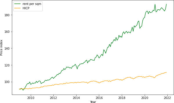
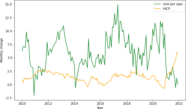
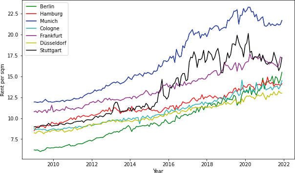
Figure 1 displays the price development presented by the monthly average rent over the observation period as well as the general price level displayed by the Harmonised Index of Consumer Prices (HICP) published by the Deutsche Bundesbank. For both factors we see a constant growth being drastically more rapid for the rent prices. While the HICP moved from 91.1 to 127.2, average rent more than doubled from 91.1 to 192.76. Figure 2 lays focus on the yearly percentage change of both variables again making clear rents strongly outpace common price developments. But there are periods when rent price growth falls behind the HICP change. We see that around 2011 and 2014. Even more evident is the period from 2021 onwards, where the common price level is poised to exceed rents in the midterm. Figure 3 looks at prices over time periods across cities. By far the most expensive city over the whole period is Munich, followed by Frankfurt am Main and Stuttgart, which has seen a tremendous price increase from 2016 onwards. The remaining cities move in the same price range although Berlin is coming from a far lower starting point and has made a strong ascent.
In summary the data behaves as we would expect from a real estate dataset of the seven biggest cities in Germany and there were no conspicuous inconsistencies. Finally, the dataset was split into an 80% training set and a 20% testing set.
Although not the focus of our predictive study, residuals are an essential aspect, as they guide us in model improvements and ensure robust, reliable predictions. The literature on real estate price forecasts models, which focuses on model performance applies various residual metrics besides RMSE. And although they use metrics like Mean Absolute Error (MAE), Mean Squared Error (MSE), R-squared or Adjusted R-squared, RMSE is widely used for its comparability, error magnification and standard practice. Given its properties, RMSE provides a single, interpretable measure of model error in the same units as the predicted variable, making it particularly useful for communicating results to diverse stakeholders. While other metrics like MAE emphasize absolute deviations and R-squared measures goodness-of-fit, RMSE effectively balances by penalizing larger errors more heavily, offering insight into model performance under typical use scenarios. Consequently, for the purpose of our study, relying solely on RMSE is both practical and justified.
Table 3 summarizes the RMSE for all training and testing results. We initiate our analysis by training a standard OLS model. The RMSE for the training set is 2.96, while it is 2.95 for the test set. Subsequently, we apply statistical filters to address potential overfitting caused by superfluous variables. We apply correlation-based feature selection, k-best method, and low variance filters, but none demonstrate an improvement in the OLS model.
| LR | Dt | XGB | ||
|---|---|---|---|---|
| RMSE | train | 2.90 | 2.74 | 2.08 |
| test | 2.89 | 2.75 | 2.12 |
To introduce non-linearity, we incorporate squared and interaction terms based on univariate analysis. Squaring minimally improves the model (RMSE: 2.90 (train), 2.89 (test). So does including interaction terms, but to an even lower degree (RMSE: 2.94 (train), 2.94 (test)). Bootstrapping, aiming to make linear regression comparable to modern machine learning algorithms, does not yield improvements (RMSE: 2.95 (train), 2.95 (test)). Due to the at most marginal improvement through non-linearity, we retain simple OLS as our baseline model.
We further explore complexity by training a decision tree model with pruning to avoid overestimation. Hyperparameter tuning identifies optimal parameters as a maximal depth of 9 and minimal splits of 3, resulting in an RMSE of 2.74 for the training set and 2.75 for the test set.
Lastly, we employ an XGB model without hyperparameter tuning, yielding an impressive result of 2.08 for the training set and 2.12 for the test set. These findings align with established literature on ML in real estate market domain, as discussed in literature review in section 2.
5.2 SHAP analysis – preprocessing
As described in the data section (4.2), we reduce the dataset using Slovin’s Formula (Equation 10), ensuring computational feasibility without compromising representativeness. This sample size facilitates a detailed SHAP analysis while maintaining the validity of our finding. This leaves us with a sample size of 2,946 observations. SHAP values for XGB, even with reduced data, demonstrated consistent feature importance. Table 4 shows the evaluation of the deviations between the calculated SHAP values of the reduced data set, and a random sample set of 100,000 observations. The average absolute deviation between respective features is just 0.001, the largest difference is 0.02. Overall, we find only 16 out of 150 features that show any deviation at all, and of these, the deviation is only 0.01 for 13 of those features. The results confirm the chosen data reduction methodology to be valid and reliable, so that we use it as the basis for all subsequent applications of SHAP values.
| Mean Diff. (abs.) | 0.001 |
| Max Diff. (abs.) | 0.02 |
| No. non-zeros | 16 |
| No. 0.01-Diff. | 13 |
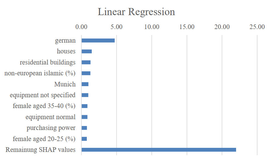
This section provides a detailed description of the insights and findings based on SHAP evaluation, culminating in a bullet-point overview at the end of the section. Figure 4 delineates that the LR model predominantly derives its predictive outcomes from the variable denoting the percentage of households with a German head (German (%)). The associated SHAP value of 4.73 markedly surpasses the subsequent significant influence, namely, the count of residential buildings (houses) (1.47). The discernible discrepancy between these two pivotal variables is comparatively diminished within the context of the decision tree. The foremost variable, namely, the share of the Muslim population (non-European Islamic (%)) (1.18), is marginally separated by a mere 0.06 from the second-ranking variable, denoting the city of Munich (1.12). Furthermore, the subsequent features contribute more significantly relative to the primary variable in comparison to the LR model. This observation also holds true for the XGB model, where the differential impact between the leading two features is quantified at 0.23 (1.01 vs. 0.78).
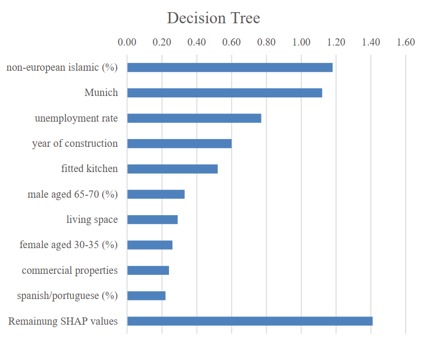
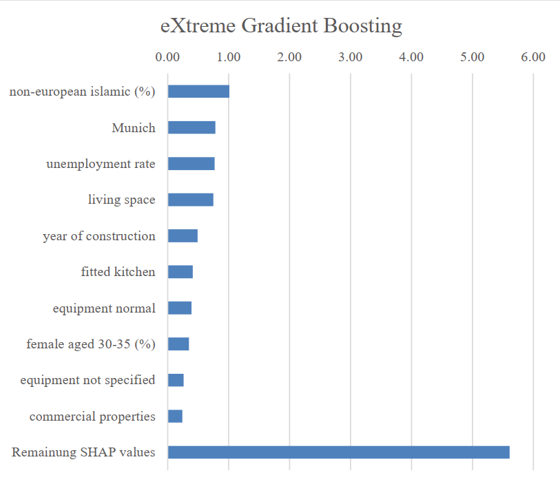
Additionally, the findings indicate a noteworthy disparity in SHAP values, with those associated with LR generally exhibiting substantially greater magnitudes than those observed for DT and XGB models. Table 5 presents the cumulative mean SHAP values (Conceição, 2023), unequivocally illustrating the pronounced preponderance of LR SHAPs (LR: 36.01; DT: 6.94; XGB: 11.06). In conjunction with our understanding that LR demonstrates inferior predictive efficacy, we can deduce that this suboptimal performance stems from the inherent granularity of individual influencing variables or in other words LR tends to overshoot in predicting the target variable.
| LR | DT | XGB | |
|---|---|---|---|
| SHAP sum | 36.01 | 6.94 | 11.06 |
Furthermore, an insightful revelation from the SHAP analysis is the comparatively diminished significance of dummy variables in LR as opposed to the other models. Table 6 provides a summation of the mean absolute SHAP values, accompanied by the percentage allocation of dummy and remaining SHAPs for each respective model (Conceição, 2023). This dual representation ensures comprehensive coverage of 100%. Notably, the proportion of dummy variable SHAPs is least prominent for LR (27%), experiencing a 5-percentage point increment for DT (32%) and further escalating by an equivalent magnitude for XGB (37%). Consequently, we observe an augmentation in the significance of dummy variables with escalating model complexity. This outcome aligns with intuition, given that dummy variables, characterized by binary states, possess inherently weak predictive prowess in comparison to continuous influencing variables, particularly in the absence of permissible interaction terms. It is pertinent to highlight that both DT and XGB, owing to their multilayered structure, facilitate multiple interactions among diverse explanatory variables. This structural attribute allows the relatively coarse predictive influence of a dummy variable to undergo refinement through its interrelation with other variables.
| LR | DT | XGB | |
|---|---|---|---|
| Dummy Variables | 9.76 (27%) | 2.20 (32%) | 4.13 (37%) |
| Non Dummy Variables | 26.25 (73%) | 4.74 (68%) | 6.93 (63%) |
Another salient feature discerned from the SHAP values is the notable disparity in the number of variables that play no role in the model, presenting a distinctive characteristic across models. Table 7 reveals that the count of features with an average absolute SHAP value of 0 is markedly elevated for the DT model at 104, in stark contrast to LR model (22) and the XGB model (25). This observation implies that DT, despite outperforming LR in predictive power with a lower RMSE, relies on fewer variables for its predictions. This would typically suggest a potential compromise in performance; however, the DT compensates by capturing more intricate interactions among relevant variables.
| LR | DT | XGB | |
|---|---|---|---|
| No. Zero-SHAPs | 22 | 104 | 25 |
In contrast, a comparable number of variables are deemed relevant for the XGB model. Given its superior performance, one can infer that the allowance for higher complexity in form of more tree layers enables the inclusion of more features, thereby enhancing performance through the utilization of even deeper trees. This is substantiated by Table 5, which illustrates that the sum of the average influence for XGB is nearly double that of DT (11.06 vs. 6.94).
The final insight directs our attention back to Figure 4, portraying the top ten most important features for each model. Examination of these top ten features for DT and XGB reveals a striking overlap. To enhance clarity, Table 8 employs colored markers to denote this overlap. Green signifies features present in the same rank for both models, while orange indicates features within the top ten but not in the same rank. The absence of color denotes variables that do not appear in the other model’s top ten. The prevalence of green and orange fields underscores the robust concordance between the two models. Notably, the four features lacking counterparts endorse the notion that a more complex model adeptly accommodates dummy variables. This distinction arises as DT relies on two additional continuous variables (male aged 65-75 (%) and Spanish Portuguese (%)), whereas XGB achieves a similar effect through the inclusion of the two dummy variables, equipment normal and equipment not specified.
| Rank | DT | XGB | |||||||||||||||||
|---|---|---|---|---|---|---|---|---|---|---|---|---|---|---|---|---|---|---|---|
| 1 | non-European Islamic (%)* | non-European Islamic (%)* | |||||||||||||||||
| 2 | Munich* | Munich* | |||||||||||||||||
| 3 | unemployment rate* | unemployment rate* | |||||||||||||||||
| 4 | year of construction# | living space# | |||||||||||||||||
| 5 | fitted kitchen# | year of construction# | |||||||||||||||||
| 6 | male aged 65-75 (%) | fitted kitchen# | |||||||||||||||||
| 7 | living space# | equipment normal | |||||||||||||||||
| 8 | female aged 30-35 (%)* | female aged 30-35 (%)* | |||||||||||||||||
| 9 | commercial properties# | equipment Not specified | |||||||||||||||||
| 10 | Spanish Portuguese (%) | commercial properties# | |||||||||||||||||
| Note: symbols are utilized to represent the overlap between the top 10 features between DT and XGB models. * indicates features sharing the same rank, # features within the top ten but with differing ranks, and no symbol features not appearing in other top 10. | |||||||||||||||||||
To summarize our results on model interpretability, our comparative analysis across LR, DT, and XGB models unveiled five compelling conclusions:
1. Variable Importance:
–LR heavily relies on a single major variable, while ML models exhibit a broader perspective.
–Dummy variables gain importance with model complexity.
2. SHAP Magnitudes:
–LR SHAP values are higher, yet its performance is inferior to ML models.
3. Dummy Variable Significance:
–Dummy variable importance increases with model complexity, especially evident in DT and XGB.
4. Model Complexity and Relevant Variables
–A kind of U-shape relationship exists between model complexity and the number of relevant variables.
–Top features for tree-based ML models (DT and XGB) are strikingly similar.
5. Number of Variables Playing a Role:
–DT relies on fewer variables with high predictive power, whereas XGB embraces complexity, incorporating more features for enhanced performance.
Our meticulous analysis not only highlights the strengths and weaknesses of each model but also provides valuable insights into the nuanced interplay between model complexity, variable significance, and predictive accuracy. With a focus on practical applications and alignment with existing literature, this study offers a compelling blueprint for leveraging advanced modeling techniques in real estate market analysis. The results are not just numbers; they are a gateway to a deeper understanding of the intricate relationships that govern real estate dynamics, unlocking new possibilities for informed decision-making in the ever-evolving market landscape.
In this comprehensive analysis of predictive modeling for real estate market forecasting, our findings highlight the strengths and limitations of various techniques. Traditional linear approaches, such as OLS, prove to be suboptimal, with non-linearity introduced through squared and interaction terms failing to significantly improve predictive performance. DT models offer a notable improvement, particularly when pruned to avoid overestimation, but it is the XGB that emerges as the most promising, aligning with existing literature in real estate markets. The SHAP analysis provides valuable insights into the interpretability of these models, revealing patterns in variable importance and the impact of model complexity on the significance of dummy variables.
Beyond the technical findings, this study also offers practical insights into the drivers of rental prices in the German residential market. These results can provide a valuable foundation for public policy discussions, particularly in addressing housing affordability and urban planning challenges. For instance, the identified key features influencing rental prices can guide government initiatives aimed at regulating rents or improving housing market transparency. While the primary aim of this paper was methodological, the results themselves offer actionable insights that warrant further exploration, particularly in collaboration with public institutes and stakeholders.
For future research deeper investigations into the implications of these results, especially regarding policy impacts and regional disparities, can enrich the field. Exploring the interaction between identified predictors and broader socioeconomic trends as well as extending the application of interpretable machine learning models to other real estate contexts, can further enhance the utility of these findings. By sharing this analysis with public governments or non-profit organizations, we align with the broader mission of contributing to societal well-being through impactful research.
Adadi, A., & Berrada, M. (2018). Peeking inside the black-box: a survey on explainable artificial intelligence (XAI). IEEE access, 6, 52138–52160.
Ahlfeldt, G. M., Redding, S. J., Sturm, D. M., & Wolf, N. (2015). The economics of density: evidence from the Berlin Wall. Econometrica, 83(6), 2127–2189.
Alfano, V., & Guarino, M. (2022). A word to the wise analyzing the impact of textual strategies in determining house pricing. Journal of Housing Research, 31(1), 88–112.
Allard, N., & Hagström, T. (2021). Modern housing valuation: a machine learning approach. Degree project in industrial engineering and management.
Al-Qawasmi, J. (2022). Machine learning applications in real estate: critical review of recent development. In Maglogiannis, I., Iliadis, L., Macintyre, J., & Cortez, P. (Eds.). Artificial Intelligence Applications and Innovations. AIAI 2022. IFIP Advances in Information and Communication Technology, Vol. 647. Cham, Springer.
Alsawan, N. M., & Alshurideh, M. T. (2022). The application of artificial intelligence in real estate valuation: a systematic review. In Hassanien, A. E., Snášel, V., Tang, M., Sung, T. W., & Chang, K. C. (Eds.). Proceedings of the 8th International Conference on Advanced Intelligent Systems and Informatics 2022. AISI 2022. Lecture Notes on Data Engineering and Communications Technologies, Vol. 152. Cham, Springer.
Antipov, E. A., & Pokryshevskaya, E. B. (2012). Mass appraisal of residential apartments: an application of Random forest for valuation and a CART-based approach for model diagnostics. Expert Systems with Applications, 39(2), 1772–1778.
Athey, S., & Imbens, G. W. (2019). Machine learning methods that economists should know about. Annual Review of Economics, 11, 685–725.
Awonaike, A., Ghorashi, S. A., & Hammaad, R. (2021, December). A machine learning framework for house price estimation. In Abraham, A., Gandhi, N., Hanne, T., Hong, T. P., Nogueira Rios, T., & Ding, W. (Eds.). Intelligent Systems Design and Applications. ISDA 2021. Lecture Notes in Networks and Systems, Vol. 418. Cham, Springer.
Baur, K., Rosenfelder, M., & Lutz, B. (2023). Automated real estate valuation with machine learning models using property descriptions. Expert Systems with Applications, 213, 119147.
Beimer, J., & Francke, M. (2019). Out-of-sample house price prediction by hedonic price models and machine learning algorithms. Real Estate Research Quarterly, 18(2), 13–20.
Below, S., Beracha, E., & Skiba, H. (2015). Land erosion and coastal home values. Journal of Real Estate Research, 37(4), 499–536.
Blackley, D. M., Follain, J. R., & Lee, H. (1986). An evaluation of Hedonic Price Indexes for thirty‐four large SMSAs. Real Estate Economics, 14(2), 179–205.
Breidenbach, P., & Eilers, L. (2018). RWI-GEO-GRID: Socio-economic data on grid level. Jahrbücher für Nationalökonomie und Statistik, 238(6), 609–616.
Breiman, L. (1997). Arcing the edge. Technical Report 486, pp. 1-14, Statistics Department, University of California at Berkeley.
Breiman, L. (2003). Statistical modeling: The two cultures. Quality Control and Applied Statistics, 48(1), 81–82.
Breuer, W., & Steininger, B. I. (2020). Recent trends in real estate research: a comparison of recent working papers and publications using machine learning algorithms. Journal of Business Economics, 90, 963–974.
Cajias, M., Willwersch, J., Lorenz, F., & Schaefers, W. (2021). Rental pricing of residential market and portfolio data–A hedonic machine learning approach. Real Estate Finance, 38(1), 1–17.
Can, A. (1992). Specification and estimation of hedonic housing price models. Regional Science and Urban Economics, 22(3), 453–474.
Carvalho, D. V., Pereira, E. M., & Cardoso, J. S. (2019). Machine learning interpretability: a survey on methods and metrics. Electronics, 8(8), 832.
Chan, K. W., & Chin, T. L. (2002). A critical review of literature on the hedonic price model and its application to the housing market in Penang. In The Seventh Asian Real Estate Society Conference, Seul (p. 12).
Chen, T., & Guestrin, C. (2016). Xgboost: a scalable tree boosting system. In Proceedings of the 22nd ACM SIGKDD International Conference on Knowledge Discovery and Data Mining (KDD ‘16). Association for Computing Machinery, New York, NY, USA, 785–794.
Chen, J. H., Ong, C. F., Zheng, L., & Hsu, S. C. (2017). Forecasting spatial dynamics of the housing market using support vector machine. International Journal of Strategic Property Management, 21(3), 273–283.
Chernobai, E., Reibel, M., & Carney, M. (2011). Nonlinear spatial and temporal effects of highway construction on house prices. The Journal of Real Estate Finance and Economics, 42, 348–370.
Chin, S., Kahn, M. E., & Moon, H. R. (2020). Estimating the gains from new rail transit investment: a machine learning tree approach. Real Estate Economics, 48(3), 886–914.
Chun Lin, C., & Mohan, S. B. (2011). Effectiveness comparison of the residential property mass appraisal methodologies in the USA. International Journal of Housing Markets and Analysis, 4(3), 224–243.
Colwell, P. F., & Dilmore, G. (1999). Who was first? An examination of an early hedonic study. Land Economics, 620–626.
Conceição, R. Q. (2023). Supervised clustering with SHAP values. Doctoral dissertation, Instituto Superior de Economia e Gestão, Universidade de Lisboa.
Connellan, O., & James, H. (1998). Estimated realisation price (ERP) by neural networks: forecasting commercial property values. Journal of Property Valuation and Investment, 16(1), 71–86.
Conway, D., Li, C. Q., Wolch, J., Kahle, C., & Jerrett, M. (2010). A spatial autocorrelation approach for examining the effects of urban greenspace on residential property values. The Journal of Real Estate Finance and Economics, 41, 150–169.
Court, A. T. (1939). Hedonic price indexes with automotive examples. In The dynamics of automobile demand (pp. 99–117). New York, General Motors Corporation.
Craven, M., & Shavlik, J. (1995). Extracting tree-structured representations of trained networks. In Advances in Neural Information Processing Systems 8 (NIPS 1995), pp. 24–30.
Deaconu, A., Buiga, A., & Tothăzan, H. (2022). Real estate valuation models performance in price prediction. International Journal of Strategic Property Management, 26(2), 86–105.
Delgado-Panadero, Á., Hernández-Lorca, B., García-Ordás, M. T., & Benítez-Andrades, J. A. (2022). Implementing local-explainability in gradient boosting trees: feature contribution. Information Sciences, 589, 199–212.
Des Rosiers, F., Dubé, J., & Thériault, M. (2011). Do peer effects shape property values?. Journal of Property Investment & Finance, 29(4/5), 510–528.
Dubin, R. A. (1988). Estimation of regression coefficients in the presence of spatially autocorrelated error terms. The Review of Economics and Statistics, 466–474.
Duell, J., Fan, X., Burnett, B., Aarts, G., & Zhou, S. M. (2021). A comparison of explanations given by explainable artificial intelligence methods on analysing electronic health records. In 2021 IEEE EMBS International Conference on Biomedical and Health Informatics (BHI), pp. 1–4. IEEE.
Dumm, R. E., Sirmans, G. S., & Smersh, G. T. (2016). Price variation in waterfront properties over the economic cycle. Journal of Real Estate Research, 38(1), 1–26.
Dumm, R. E., Sirmans, G. S., & Smersh, G. T. (2018). Sinkholes and residential property prices: Presence, proximity, and density. Journal of Real Estate Research, 40(1), 41–68.
Dunse, N., & Jones, C. (2002). The existence of office submarkets in cities. Journal of Property Research, 19(2), 159–182.
Fernández-Avilés, G., Minguez, R., & Montero, J. M. (2012). Geostatistical air pollution indexes in spatial hedonic models: the case of Madrid, Spain. Journal of Real Estate Research, 34(2), 243–274.
Fisher, A., Rudin, C., & Dominici, F. (2019). All models are wrong, but many are useful: learning a variable’s importance by studying an entire class of prediction models simultaneously. Journal of Machine Learning Research, 20(177), 1-81.
Friedman, J. H. (2001). Greedy function approximation: a gradient boosting machine. Annals of Statistics, 29(5), 1189–1232.
Foryś, I. (2022). Machine learning in house price analysis: regression models versus neural networks. Procedia Computer Science, 207, 435–445.
Goodwin, K. R., La Roche, C. R., & Waller, B. D. (2020). Restrictions versus amenities: the differential impact of home owners associations on property marketability. Journal of Property Research, 37(3), 238–253.
Grybauskas, A., Pilinkienė, V., & Stundžienė, A. (2021). Predictive analytics using Big Data for the real estate market during the COVID-19 pandemic. Journal of Big Data, 8(1), 1–20.
Guliker, E., Folmer, E., & van Sinderen, M. (2022). Spatial determinants of real estate appraisals in the Netherlands: A machine learning approach. ISPRS international journal of geo-information, 11(2), 125.
Haas, G. C. (1922). Sale prices as a basis for farmland appraisal. Technical Bulletin, Vol. 9. University Farm.
Hamilton, S. E., & Morgan, A. (2010). Integrating lidar, GIS and hedonic price modeling to measure amenity values in urban beach residential property markets. Computers, Environment and Urban Systems, 34(2), 133–141.
Harfitalia, P., Pujangkoro, S., & Fachrudin, H. T. (2022). Analysis of Factors Affecting the Value of Shophouse in Lubuk Pakam City, Deli Serdang Regency. International Journal of Research and Review, 9(3), 113–118.
Hastie, T., Tibshirani, R., & Priedman, J. H. (2001). The Elements of Statistical Learning. Data Mining, Inference, and Prediction. New York, Springer.
Hoen, B., & Atkinson-Palombo, C. (2016). Wind turbines, amenities and disamenitites: a study of home value impacts in densely populated Massachusetts. Journal of Real Estate Research, 38(4), 473–504.
Huang, T., & Yu, Y. (2014). Sell probabilistic goods? A behavioral explanation for opaque selling. Marketing Science, 33(5), 743–759.
Hui, E. C., Chau, C. K., Pun, L., & Law, M. Y. (2007). Measuring the neighboring and environmental effects on residential property value: Using spatial weighting matrix. Building and Environment, 42(6), 2333–2343.
Iban, M. C. (2022). An explainable model for the mass appraisal of residences: the application of tree-based Machine Learning algorithms and interpretation of value determinants. Habitat International, 128, 102660.
Isakson, H. (2002). The linear algebra of the sales comparison approach. Journal of Real Estate Research, 24(2), 117–128.
James, G., Witten, D., Hastie, T., & Tibshirani, R. (2013). An introduction to statistical learning. Vol. 112, p. 18. New York, Springer.
Jauregui, A., Allen, M. T., & Weeks, H. S. (2019). A spatial analysis of the impact of float distance on the values of canal-front houses. Journal of Real Estate Research, 41(2), 285–318.
Katzenbeisser, S., & Petitcolas, F. (2016). Information hiding. Artech house.
Khosravi, M., Arif, S. B., Ghaseminejad, A., Tohidi, H., & Shabanian, H. (2022). Performance evaluation of machine learning regressors for estimating real estate house prices. Available at: https://www.preprints.org/manuscript/202209.0341 (accessed 11 December 2023).
Knight, J., Sirmans, C., & Turnbull, G. (1998). List price information in residential appraisal and underwriting. Journal of Real Estate Research, 15(1), 59–76.
Kok, N., Koponen, E. L., & Martínez-Barbosa, C. A. (2017). Big data in real estate? From manual appraisal to automated valuation. The Journal of Portfolio Management, 43(6), 202–211.
Konstantinov, A. V., & Utkin, L. V. (2021). Interpretable machine learning with an ensemble of gradient boosting machines. Knowledge-Based Systems, 222, 106993.
Kontrimas, V., & Verikas, A. (2011). The mass appraisal of the real estate by computational intelligence. Applied Soft Computing, 11(1), 443–448.
Krämer, B., Nagl, C., Stang, M., & Schäfers, W. (2023). Explainable AI in a real estate context–exploring the determinants of residential real estate values. Journal of Housing Research, 32(2), 204–245.
Kumar, C. S., Choudary, M. N. S., Bommineni, V. B., Tarun, G., & Anjali, T. (2020). Dimensionality reduction based on shap analysis: a simple and trustworthy approach. In 2020 International Conference on Communication and Signal Processing (ICCSP), Chennai, India, 2020, pp. 558-560. IEEE. 2020,
Kumkar, P., Madan, I., Kale, A., Khanvilkar, O., & Khan, A. (2018). Comparison of ensemble methods for real estate appraisal. In 2018 3rd International Conference on Inventive Computation Technologies (ICICT), Coimbatore, India, pp. 297-300. IEEE.
Lancaster, K. J. (1966). A new approach to consumer theory. Journal of Political Economy, 74(2), 132–157.
Linardatos, P., Papastefanopoulos, V., & Kotsiantis, S. (2020). Explainable ai: a review of machine learning interpretability methods. Entropy, 23(1), 18.
Lorenz, F., Willwersch, J., Cajias, M., & Fuerst, F. (2023). Interpretable machine learning for real estate market analysis. Real Estate Economics, 51(5), 1178–1208.
Lundberg, S. M., & Lee, S. I. (2017). A unified approach to interpreting model predictions. In Advances in neural information processing systems 30 (NIPS 2017).
Lundberg, S. M., Erion, G., Chen, H., DeGrave, A., Prutkin, J. M., Nair, B., Katz, R., Himmelfarb, J., Bansal, N., & Lee, S. I. (2019). Explainable AI for trees: from local explanations to global understanding. arXiv preprint arXiv:1905.04610.
Malpezzi, S. (2003). Hedonic pricing models: a selective and applied review. In O’Sullivan, T., & Gibb, K. (Eds.). Housing Economics and Public Policy, 67–89. Oxford, Blackwell.
Mayer, M., Bourassa, S. C., Hoesli, M., & Scognamiglio, D. (2019). Estimation and updating methods for hedonic valuation. Journal of European Real Estate Research, 12(1), 134–150.
McCluskey, W., Davis, P., Haran, M., McCord, M., & McIlhatton, D. (2012). The potential of artificial neural networks in mass appraisal: the case revisited. Journal of Financial Management of Property and Construction, 17(3), 274–292.
Merrick, L., & Taly, A. (2020). The explanation game: explaining machine learning models using shapley values. In Machine Learning and Knowledge Extraction: 4th IFIP TC 5, TC 12, WG 8.4, WG 8.9, WG 12.9 International Cross-Domain Conference, CD-MAKE 2020, Dublin, Ireland, August 25–28, 2020, Proceedings 4, 17–38. Springer International Publishing.
Merrick, L., Taly, A. (2020). The Explanation Game: Explaining Machine Learning Models Using Shapley Values. In: Holzinger, A., Kieseberg, P., Tjoa, A., Weippl, E. (eds) Machine Learning and Knowledge Extraction. CD-MAKE 2020. Lecture Notes in Computer Science (), vol 12279. Springer, Cham.
Molnar, C. (2022). Interpretable machine learning: a guide for making black box models explainable. 2nd ed. Lulu.com.
Morgan, J. N., & Sonquist, J. A. (1963). Some results from a non-symmetrical branching process that looks for interaction effects. Young, 8(5).
Pace, R. K., & Hayunga, D. (2020). Examining the information content of residuals from hedonic and spatial models using trees and forests. The Journal of Real Estate Finance and Economics, 60, 170–180.
Pérez-Rave, J. I., Correa-Morales, J. C., & González-Echavarría, F. (2019). A machine learning approach to big data regression analysis of real estate prices for inferential and predictive purposes. Journal of Property Research, 36(1), 59–96.
Piegeler, T., Bauer, S., Ondrusch, S., & von Ditfurth, J. (2021). Knowing what others don’t: gaining a competitive edge in real estate with AI-driven geospatial analytics. Deloitte Insights. Available at: www2. deloitte.com/uk/en/pages/realestate/articles/gaining-a-competitive-edge-in-real-estate.html (accessed 31 August 2023).
Quinlan, J. R. (1979). Discovering rules by induction from large collections of examples. Expert systems in the micro electronics age. Edinburgh, Edinburgh University Press.
Rosen, S. (1974). Hedonic prices and implicit markets: product differentiation in pure competition. Journal of Political Economy, 82(1), 34–55.
Rouwendal, J., Levkovich, O., & Van Marwijk, R. (2017). Estimating the value of proximity to water, when ceteris really is paribus. Real Estate Economics, 45(4), 829–860.
Ryan, T. P. (2013). Sample size determination and power. Hoboken, John Wiley & Sons.
Samek, W. (2020). Learning with explainable trees. Nature Machine Intelligence, 2(1), 16–17.
Sangani, D., Erickson, K., & Al Hasan, M. (2017). Predicting zillow estimation error using linear regression and gradient boosting. In 2017 IEEE 14th International Conference on Mobile Ad Hoc and Sensor Systems (MASS), Orlando, FL, USA, pp. 530–534. IEEE.
Schaffner, S., & Boelmann, B. (2018). FDZ Data description: Real-Estate Data for Germany (RWI-GEO-RED)-Advertisements on the Internet Platform ImmobilienScout24. RWI Projektberichte, RWI. Leibniz-Institut für Wirtschaftsforschung, Essen
Schaffner, S., & Thiel, P. (2022). FDZ data description: Real-estate data for Germany (RWI-GEO-RED v7)-Advertisements on the internet platform lmmobilienScout24 2007-06/2022. RWI Datenbeschreibung. RWI – Leibniz-Institut für Wirtschaftsforschung, Essen
Shen, L., & Springer, T. M. (2022). The odd one out? the impact of property uniqueness on selling time and selling price. Journal of Housing Research, 31(2), 220–240.
Singh, A., Sharma, A., & Dubey, G. (2020). Big data analytics predicting real estate prices. International Journal of System Assurance Engineering and Management, 11, 208–219.
Sirmans, S., Macpherson, D., & Zietz, E. (2005). The composition of hedonic pricing models. Journal of Real Estate Literature, 13(1), 1–44.
Stang, M., Krämer, B., Nagl, C., & Schäfers, W. (2023). From human business to machine learning—methods for automating real estate appraisals and their practical implications. Zeitschrift Für Immobilienökonomie, 9(2), 81–108.
Stamou, M., Mimis, A., & Rovolis, A. (2017). House price determinants in Athens: a spatial econometric approach. Journal of Property Research, 34(4), 269–284.
Sundararajan, M., & Najmi, A. (2020). The many Shapley values for model explanation. In Proceedings of the 37th International Conference on Machine Learning, 9269–9278. PMLR.
Suparman, Y., Folmer, H., & Oud, J. H. (2014). Hedonic price models with omitted variables and measurement errors: a constrained autoregression–structural equation modeling approach with application to urban Indonesia. Journal of Geographical Systems, 16, 49–70.
Surkov, A., Srinivas, V., & Gregorie, J. (2022). Unleashing the power of machine learning models in banking through explainable artificial intelligence (XAI). Deloitte Insights. Available at: https://www2.deloitte.com/us/en/insights/industry/financial-services/explainable-ai-in-banking.html (accessed 31 August 2023).
Tekin, M., & Sari, I. U. (2022). Real Estate Market Price Prediction Model of Istanbul. Real Estate Management and Valuation, 30(4), 1–16.
Theisen, T., & Emblem, A. W. (2018). House prices and proximity to kindergarten–costs of distance and external effects?. Journal of Property Research, 35(4), 321–343.
Ünel, F. B., & Yalpir, S. (2019). Reduction of mass appraisal criteria with principal component analysis and integration to GIS. International Journal of Engineering and Geosciences, 4(3), 94–105.
Valier, A. (2020). Who performs better? AVMs vs hedonic models. Journal of Property Investment & Finance, 38(3), 213–225.
Wang, D., & Li, V. J. (2019). Mass appraisal models of real estate in the 21st century: a systematic literature review. Sustainability, 11(24), 7006.
Wyman, D., & Mothorpe, C. (2018). The pricing of power lines: a geospatial approach to measuring residential property values. Journal of Real Estate Research, 40(1), 121–154.
Yavas, A., & Yang, S. (1995). The strategic role of listing price in marketing real estate: theory and evidence. Real Estate Economics, 23(3), 347–368.
Yilmazer, S., & Kocaman, S. (2020). A mass appraisal assessment study using machine learning based on multiple regression and random forest. Land Use Policy, 99, 104889.
Yoo, S., Im, J., & Wagner, J. E. (2012). Variable selection for hedonic model using machine learning approaches: a case study in Onondaga County, NY. Landscape and Urban Planning, 107(3), 293–306.
Zurada, J., Levitan, A., & Guan, J. (2011). A comparison of regression and artificial intelligence methods in a mass appraisal context. Journal of Real Estate Research, 33(3), 349–388.
| Category | Variable | Description | Analyis element within attribute | Variable type |
|---|---|---|---|---|
| RED | ||||
| Price information | rent per sqm | Exclusive rent per squared meter | Euro per sqm | Contiuous |
| Object features | year of construction | Year that object was built | Integer (Number of year) | continous |
| living space | Living area | Number of square meters | continous | |
| floor | Floor on which object is located | Integer between -1 and 45 | continous | |
| number of rooms | Number of rooms | Integer between 0.5 and 10 | continous | |
| elevator | Elevator in object | Existence: Yes/No | categorical (dummy) | |
| balcony | Balcony at object | Existence: Yes/No | categorical (dummy) | |
| assisted living | Assisted living for the elderly | Existence: Yes/No | categorical (dummy) | |
| listed building | Protected historic building | Existence: Yes/No | categorical (dummy) | |
| fitted kitchen | Kitchenette in object | Existence: Yes/No | categorical (dummy) | |
| public housing | Public housing – certificate of eligibility is needed | Existence: Yes/No | categorical (dummy) | |
| guest toilet | Guest toilet in object | Existence: Yes/No | categorical (dummy) | |
| garden | (Shared) garden available | Existence: Yes/No | categorical (dummy) | |
| cellar | Cellar in object | Existence: Yes/No | categorical (dummy) | |
| parking lot | Garage/ parking space available | Existence: Yes/No | categorical (dummy) | |
| wheelchair accessible | Accessible, no steps | Existence: Yes/No | categorical (dummy) | |
| equipment | Facilities of object | Existence: Not specified, Normal, Sophisticated, Deluxe, Simple | categorical | |
| Energy and structure information | energy efficiency class | Energy Efficiency Rating | Existence: Not specified, D, E, B, C, A, G, F, APLUS, H | categorical |
| energy certificate type | Type of Energy Performance Certificates (EPCs) | Existence: Not specified, Energy use [Energieverbauchskennwert], Energy demand [Energiebedarf] | categorical | |
| type of heating | Type of heating | Energy Generation Systems · Gas heating · Oil heating · Thermal heat pump · Electric heating · Cogeneration/combined heat and power plant · Wood pellet heating · Solar heating Energy Delivery Systems · Central heating · Self-contained central heating · Heating by stove · District heating · Night storage heaters · Floor heating |
categorical | |
| property condition | Condition of object | New Buildings · First occupancy · Like new · First occupancy after reconstruction Existing Buildings · Completely renovated · Modernised · Well kept · Not specified · Reconstructed · Needs renovation · By arrangement · Dilapidated |
categorical | |
| Regional information | gid2015 | Municipality identifier (AGS, 2015) | Existence: Berlin, Hamburg, Munich, Cologne, Frankfurt, Stuttgart, Düsseldorf | categorical |
| Time period | year | Beginning of ad, year | Integer (Number of year) | continous |
| month | Beginning of ad, month | Integer (Number of month) | continous | |
| GRID | ||||
| Neighborhood information | Number of households | Absolute number | Integer | continuous |
| Number of commercial enterprises | Absolute number | Integer | continuous | |
| Number of houses (including pure commercial buildings) | Absolute number | Integer | continuous | |
| Number of residential buildings (excluding pure commercial buildings) | Absolute number | Integer | continuous | |
| Building Development | House type | Percentage per household | % | percentage |
| Household | Purchasing power | In Euro | Euro | continuous |
| Household structure | Percentage per household | % | percentage | |
| Children | Number per household | % | percentage | |
| Unemployment | rate Share of the unemployed in the population | % | percentage | |
| Ethno | Percentage of households | % | percentage | |
| Foreigners | Percentage of households | % | percentage | |
| Payment default | Percentage of households | % | percentage | |
| Population | Gender and age structure | Share of inhabitants w.r.t. sex and 17 age groups | % | percentage |
| Population structure | Absolute number of inhabitants | % | percentage |
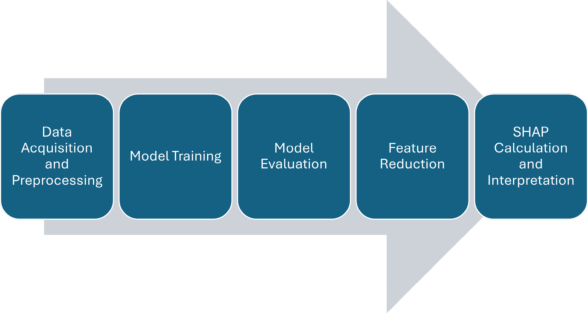
1 As we show in our literature review (section 2) the segmentation of real estate markets into submarkets is predominantly driven by the influence of location. Location-specific attributes, such as proximity to central business districts, transportation hubs or other neighborhood characteristics play a crucial role in shaping real estate values.