Property valuation: a comparative analysis of innovative market approach methods
1 Department of Architecture and Design, Sapienza University of Rome, Rome, Italy
2 Department of Industrial Engineering, University of Naples Federico II, Naples, Italy
E-mail: francesco.tajani@uniroma1.it; pierfrancesco.depaola@unina.it; giuseppe.cerullo@uniroma1.it
*Corresponding author
Abstract. This research aims to illustrate and implement innovative methods for property valuation, by comparing their respective outcomes in terms of statistical accuracy and empirical reliability. In particular, the paper describes and compares three market approach methods through an application to a case study located in the city of Rome (Italy), in order to outline their ability to rationalise the assessment in dynamic contexts and minimise the professional valuer’s subjectivity. This work represents a new reference for valuers, in order to refine their estimates and guarantee transparency in their use, avoiding the risk of black boxes that frequently characterizes mass appraisal techniques (e.g. neural networks, genetic algorithms, multiple regressions, etc.), for which constant updating of the database originating the price functions would be necessary to appropriately describe the current market conditions.
Keywords: property valuation methods, real estate market value, similarity coefficients, reliability coefficients, goal programming, maximum entropy principle, Lagrange multipliers.
JEL codes: C61, R30.
Index
4.1. General Appraisal System (SGA)
4.2. The Optimized Weighted Appraisal System Method (OWASM)
4.3. Maximum Entropy Principle and Lagrange Multipliers (MAXENT)
5.5. Application of the MAXENT
In recent years, the real estate market has experienced periods of deep uncertainty, initially caused by the economic crisis linked to the pandemic COVID-19 and the consequent restrictive measures, and subsequently exacerbated by the current conflict between Russia and Ukraine. This emergency context has led to significant global volatility, with potential substantial repercussions on the real estate sector in terms of sales and prices (Kroll, 2024). In light of these dynamics, it is crucial to manage uncertainty in order to prevent or, at least, reduce the likelihood of systemic crises in financial and economic markets, as occurred with the USA subprime mortgage crisis in 2007. In this regard, Aronsohn emphasizes that uncertainty, even under “normal” conditions, is intrinsic to most market evaluations, as there is rarely a single reference price for property valuation (Aronsohn, 2020). Indeed, for each asset, the appraiser must identify the optimal combination of comparable sales, i.e., those that are characterized by the greatest similarities with the subject, in order to obtain the most accurate value assessment (Gabrielli and French, 2021). In the real estate appraisal process, it is therefore essential to adopt operational principles such as fairness, objectivity and legality, in order to improve the quality of the evaluations. The difference between the actual and expected market prices represents the risk associated with real estate evaluation activity. Consequently, it is necessary to increase risk awareness among professional valuers, by improving their technical skills and moral qualities. In general, it is important to establish and refine a real estate appraisal mechanism that minimizes risks, increases efficiency, and ensures healthy sector development (Sun, 2019), thus reducing the number of inappropriate evaluations and overvalued properties compared to their actual market values. The need to address uncertainty in a historical context characterized by the advancement of information technology and the availability of numerous software packages capable of handling large amounts of data, surpassing human processing and analysis capabilities, has led to a revolution in the decision-making processes. This revolution has been driven by the adoption of innovative mass appraisal models (Pagourtzi et al., 2003), such as genetic algorithms (Morano et al., 2018), spatial analysis models (Anselin and Getis, 1992), fuzzy logic (Chi Man Hui et al., 2009) and artificial neural networks (Borst, 1991). Data, a key component in all sectors of the modern economy, are also fundamental in the real estate sector. However, as the latter is traditionally fragmented and heterogeneous, it has encountered more difficulties in implementing technological innovations (Festa, 2021). Indeed, available data often do not allow for an exhaustive, scientific, descriptive and interpretative analysis of real estate markets. These problems are particularly evident in the context of the Italian property market, which is characterised by limited competitiveness, a lack of transparency and the absence of complete and systematic surveys of data on the characteristics of properties and the actual prices of purchases, sales and rents (De Paola, 2024). This context makes it difficult to implement econometric procedures capable of adequately describing the price formation mechanisms of properties in specific markets (Tajani and Morano, 2018). Therefore, it is necessary to adopt “hybrid” evaluation models that, even in the presence of few comparative data, can provide sufficiently objective results independent of the appraiser’s parameters, thus ensuring effective and accurate property price evaluations and improving the assessment reliability of professional valuers’ reports (Domian et al., 2015).
The paper is structured as follows. Section 3 analyzes the main literature related to the rationalization of the comparable transactions’ method. Section 4 describes in detail the SGA, the OWASM and the MAXENT. Section 5 applies the three methods to a case study, consisting of a sample of residential units located in the city of Rome (Italy). Section 6 discusses the different outputs of the three methods’ implementation, by highlighting the potentialities and the limits of each one of them. Finally, in Section 7 the conclusions are drawn, summarizing the main results obtained and the possible future implications.
In the outlined framework, the present research aims to compare three market approach methods through an implementation to an Italian case study, by highlighting the potentialities and the limits of each one of them. The first method is the General Appraisal System (SGA), which is already well-known in the relevant scientific literature (Simonotti, 2006), as listed among the main market approach methods to be used at single property asset level by numerous Italian public and private entities guidelines as a method that respects the principles of European and International Valuation Standards (Agenzia del Territorio, 2011; Associazione Bancaria Italiana, 2024; Organismo Italiano di Valutazione, 2015). The SGA is able to automatically appraise both the property values and the implicit prices of the influencing factors, without any subjective and external assumption on the parameter contributions. Through the resolution of a linear system of equations, the SGA allows an endogenous assessment of the adjustment coefficients of the comparable selling prices. The second method is the Optimised Weighted Appraisal System Method (OWASM) and represents an evolution of the SGA, as it overcomes some limitations concerning the possible linear dependency relationships in the coefficients’ matrix and the frequent low empirical reliability of the implicit prices. The third method (MAXENT) (De Paola, 2024), is based on the integration of the Maximum Entropy Principle with Lagrange multipliers and represents an innovative and powerful tool for addressing the challenges currently facing the field of real estate appraisals. This principle is founded upon the notion that, in the presence of specific observed constraints, the probability distribution that is selected should be that which maximises the uncertainty, facilitating the natural development of statistical models that are optimised for entropy (Jaynes, 1957; Shannon, 1948). Nevertheless, as will be discussed, the practical difficulty of precisely determining the implicit prices of the individual characteristics that affect the property market value is one of the operational limitations of this method. The study aims to provide a significant contribution to the issue of reliability and logical-operational rationality in real estate evaluation procedures, regardless of the basis of value that satisfies the terms of engagement. The research proposes a potential solution to the uncertain aspects that frequently intervene in the assessment of the percentage adjustments of comparable prices. In this regard, the research represents a fundamental advancement in property valuation, as the analyzed methods require few input data and are easily implementable. Furthermore, these methods can mitigate the black box risk associated with mass appraisal techniques (e.g., neural networks, genetic algorithms, multiple regressions), which necessitate constant updating to the databases underlying price functions. Moreover, it should be outlined that the proposed methods (in particular, the OWASM and the MAXENT) can constitute an integration to the canonical market-oriented methods for ordinary properties (e.g. residential units, offices, shops, etc.) and income approach methods, as the Discounted Cash Flow Analysis generally applied for special properties (e.g. hotels, nursing homes, cinemas, retail spaces, etc.), to provide additional tools to verify the results obtained. In this way, the research represents valid support for i) professional valuers, to increase the assessment reliability of their reports, ii) banks and real estate funds management companies, to verify the adequacy of the property assessments developed by external professional valuers, to identify the most appropriate strategies of investment enhancement for the investors, to periodically update the values of the properties according to the actual and current market trends, iii) government agencies, that, to ensure the fair value of the property taxes, can quickly verify the property market values.
Over the past century, the field of real estate appraisal has evolved a range of methods to effectively compare the values of assets that share similar, though not identical, characteristics. Real estate assets are typically heterogeneous and unique resulting in market prices that are shaped by a wide range of factors, including both location and physical attributes (Forte and Rossi, 1979). It is essential that these characteristics are documented in a standardized and uniform way (Roscelli, 2014). Based on the availability of data and the selected evaluation approach, the appraiser can choose from a variety of methods outlined in the literature.
The International Valuation Standards (IVS) classifies three main approaches (IVSC, 2021): the market approach, the income approach and the cost approach. These may all be used to formulate an evaluation judgement using whatever basis of value is applicable (Arcuri et al., 2020; Glumac and Rosiers, 2020; Pagourtzi et al., 2003).
Among them, the market approach has the main advantage of providing for an objective reference – the selling prices of the comparables –, exempting the valuer from the need to appropriately justify the assumptions made on the estimation parameters adopted in the income approach (cap rate, terminal value, analysis period, etc.) and in the cost approach (depreciation functions, the market value of the area, etc.) (Tajani et al., 2020). Nevertheless, the market approach is not without its own inherent limitations.
The literature offers an extensive analysis of the comparable transactions method, also known as the sales comparison approach (SCA) method, focusing on objectifying the estimation of adjustment coefficients for comparable sale prices (Tajani et al., 2020). Several research has demonstrated that the selection of comparable properties can be affected by bias, as appraisers often overemphasize the empirical data they first encounter, while giving less weight to data acquired later (Lin and Chang, 2012). The typically small sample size used for comparison is a primary concern in this context, often resulting from periods of low market activity or from a market that is inherently thin, consistently characterized by a limited number of transactions (French and Gabrielli, 2004). Furthermore, it has been widely recognized that subjectivity and uncertainty are inherent aspects of appraisal techniques (Colwell et al., 1983; Lipscomb and Gray, 1990), especially when aligning the values of comparable properties with that of the subject property (Copiello et al., 2021). Additionally, the pronounced heterogeneity of properties within the local submarket can further intensify this challenge (LaCour-Little and Green, 1998; Tajani et al., 2020). Several researchers have proposed coefficients derived from regression analysis, employing multiple regression models as a reference for adjustments able to reduce the shortcoming of subjective judgment (Kang and Reichert, 1991; Todora and Whiterell, 2002). For instance, Colwell et al. (1983) focus on the SCA and illustrate how to derive adjustment factors using the ordinary least squares (OLS) method rather than relying on the appraiser’s judgment. This highlights how the traditional need for appraiser-derived adjustment factors can be entirely supplanted by multiple regression analysis (Isakson, 2002).
The real estate mass appraisal process, which generally relies on econometric analysis, focuses on valuing large groups of properties rather than individual assets. These methods have been extensively studied and tested, underscoring their significance. Some Authors investigate the interplay between property value, property characteristics, and urban socio-economic factors (Tajani et al., 2016, 2015), even though the implementation of regression techniques (Rossini, 2000; Yalpir et al., 2006).
However, the application of econometric methods is not always feasible. This limitation often stems from the challenges of obtaining sufficiently large and representative samples, a fundamental requirement of econometric techniques, or from the poor quality of available data. While the results may be statistically significant for understanding broader trends and general patterns across the population (Piccolo and Vitale, 1984), they often fall short when addressing specific, unique cases that inevitably arise in practical applications (Iovine, 2015).
Other studies (Borst and McCluskey, 2008; Bourassa et al., 2007; Goodman and Thibodeau, 2003) have focused on enhancing sample selection by identifying submarkets where the implicit price contributions of independent variables are more likely to be similar. For instance, Case et al. (2004) developed a two-stage method in which the residuals from a single-stage OLS model are used as predictors in the two-stage model. However, it has been noted that estimating adjustments using the traditional OLS model can be inefficient, due to errors that are not independent and identically distributed (Copiello et al., 2021). As a result, in the scientific literature alternative estimators have been explored, such as generalized least squares (GLS) procedures (Pace, 1998), and models like those proposed by Pace & Gilley (1998), which resemble spatial autoregressive (SAR) models to account for spatially correlated residuals within a single-stage model. Other Authors have proposed a variation of the SCA based on the concept of spatial weight matrices, that is a characteristic of SAR models, arguing that it has significant relationships with the geographically weighted regression (GWR) method (Borst and McCluskey, 2008). The majority of existing literature advocates for the analysis of similarity in selecting comparable properties or applying the adjustment grid method. Isakson (1988; 1986) introduced the Nearest Neighbors Appraisal Technique (NNAT), where the assessed marked value is determined by a weighted average of the actual sale prices of comparable properties. In NNAT, the weights are assigned based on a multidimensional similarity measure, giving greater weight to properties that are more closely aligned with the subject property. This approach eliminates the need to calculate adjusted sale prices for the comparables. Vandell (1991) proposed a minimum variance method for selecting and weighting comparable properties, focusing on minimizing the variance among the adjusted values of comparable sales. Gau et al. (Gau et al., 1994, 1992) extended Vandell’s approach by replacing the variance with the coefficient of variation as the measure to be minimized. In both methods, the adjusted values of comparable properties are calculated using the dollar additive technique and adjustment factors derived from OLS. Curto (2005) applied the analytic hierarchy process as a multi-parameter market approach method to better rationalize the assessment of implicit prices related to quality factors. A significant area of research deals with the use of similarity and reliability coefficients (Colwell et al., 1983; Simonotti et al., 2016), particularly in market-oriented valuation methods such as the Market Comparison Approach (MCA) (Ruggiero and Salvo, 2011; Tajani et al., 2020). These coefficients enable the expansion of the geographic area for identifying potential comparables, even including properties that exhibit a greater degree of dissimilarity (Ciuna et al., 2017). Similarity indexes are generally calculated by evaluating the differences in the descriptors of the properties being compared, while the reliability coefficient is determined by assessing the variations in their adjusted prices (Berto et al., 2020). While it is logical to assume that a larger dataset of comparable properties would lead to a more accurate appraisal, some methods based on the Maximum Entropy Principle and Lagrange multipliers suggest that a small transaction sample may suffice to achieve a reliable estimated value. Brown (2017) was the first to explore the effectiveness of entropy in addressing the inefficiencies of the real estate market, a concept further developed by Chen et al. (2020). In this context, the most recent studies have been carried out by Özdilek (2023) and De Paola (2024). In particular, Özdilek’s study examined the integration of entropy measures in property evaluations, involving the modification and integration of the triadic estimates of price, cost, and income. The results obtained led to a significant improvement in the accuracy of the value measurement. De Paola’s work explores the applicability of the Maximum Entropy Principle to real estate valuations with the support of Lagrange multipliers, emphasizing how this method can significantly enhance the evaluation precision.
This analysis demonstrates that, for valuation purposes, it is feasible to achieve accurate estimates even when market data is scarce. This can be accomplished by incorporating similarity coefficients or employing an entropic approach. Indeed, when faced with limited random data, statistical methods become impractical, and mathematical attempts frequently yield results that contradict the market evidence.
It is reasonable to assume that a larger set of comparable data leads to more accurate valuation results. However, when faced with the challenge of limited resources, it becomes essential to adopt methods that can ensure reliable outcomes despite the scarcity of available information data. In this context, the SGA, the OWASM and the MAXENT methods, which will be presented as follows, prove to be particularly effective. These methods are capable of successfully addressing this challenge, enabling the production of reliable assessments even from a limited sample of property transactions.
4.1. General Appraisal System (SGA)
The SGA serves as an evaluation model capable of ascertaining both the property value and the implicit prices of various influencing factors by solving a system of linear equations.
In the linear system of equations, the known terms are the prices of the comparable properties, while the implicit price coefficients (which are among the unknowns, along with the market value of the subject property) are derived from the differences in the corresponding characteristics between the comparables and the subject property. Therefore, in the general estimation system, the unknown variables are: the estimated price of the subject property (V) and the implicit prices of individual characteristics (pi), where the index i refers to the n real estate characteristics. The known terms consist of the prices of the comparable properties (Pj), where the index j refers to the m comparables, and the differences in the corresponding values (x) of the characteristics, calculated as (xji - x0i), where the index 0 refers to the subject property.
Thus, in comparing a generic comparable property (indexed by j) with the subject property (indexed by 0), the equation linking the price of the comparable Pj to the value of the subject property V can be expressed as a linear combination of the implicit prices and the differences in characteristics, as follows:
(1)
This equation can be formulated for each comparison between the comparable properties and the subject property, leading to the definition of a linear system of equations, where the index j ranges from 1 to n, resulting in a total of m equations.
(2)
In matrix form, Equation (2) becomes:
(3)
In which p represents the appraisal vector and P denotes the vector of known selling prices, as defined in Equations (4) and (5):
(4)
(5)
The matrix D represents the difference matrix, as defined in Equation (6), where dji=xji−x0i. It is composed of the coefficients of the unknowns, with a value of 1 assigned both to the subject property and to the differences in the values of the explanatory factors.
(6)
Within each equation, the unknown coefficients of the implicit prices are determined for each characteristic as the difference between the value of the comparable property (indexed from 1 to m) and that of the subject property (indexed as 0). The coefficient for the unknown value of the subject property is set to 1 in every equation.
The solution to this system of equations can be succinctly expressed in matrix notation as the product of the inverse of the coefficient matrix and the vector of known prices:
(7)
Depending on the characteristics of the coefficient matrix D, the following scenarios may arise:
– If the matrix of known terms is square and non-singular, meaning the determinant of D is non-zero, the system is determined. In this case, the inverse of D can be calculated, leading to a unique solution that provides both the estimated value and the unknown implicit prices.
– If the system is underdetermined (i.e., the number of equations is less than the number of unknowns, ), the solution can be obtained using the Moore-Penrose generalized inverse technique.
(8)
– Finally, if the system is overdetermined (i.e., the number of independent equations exceeds the number of unknowns, ), the solution is instead provided by the following relation:
(9)
The SGA is recognized for its compliance with International Valuation Standards and its scientific robustness. The real estate evaluations manual by Tecnoborsa (2018) integrates International Valuation Standards with Italian regulations, highlighting SGA as a key appraisal method that aligns with global best practices while addressing the specifics of the Italian context. Furthermore, numerous private guidelines and professional associations, including those cited by the Italian Revenue Agency (2011), acknowledge SGA’s deterministic and multi-parameter nature, validating its use in professional practice for its transparency and operational versatility. The SGA is also endorsed by the International Valuation Standards (2015) as a model ensuring objectivity and accuracy in property valuations.
4.2. The Optimized Weighted Appraisal System Method (OWASM)
The SGA operates effectively under the assumption of a perfectly competitive market, where sufficient data are available and transactions are transparent. However, property markets rarely meet these conditions, as monopolistic competition is more commonly observed. Consequently, the SGA can only produce reliable results when a substantial amount of comparable data is accessible. In contrast, in atypical markets or when data are scarce, the SGA may lead to uncertain outcomes. Therefore, the innovation of the OWASM lies in the introduction of similarity and reliability measurements as weighting coefficients in the SGA equation system, allowing to assign different importance to the comparables according to their respective degrees of similarity and reliability.
One measure that can be used to assess the similarity of individual properties within a sample of properties is based on the ‘closeness’ of their respective explanatory factors. In other words, greater comparability corresponds to closer proximity in the values of the property characteristics, while less comparability indicates greater differences among these values. Consequently, the ‘degree of similarity’ of comparable properties can be expressed as a function of the difference between the i-th characteristic of a comparable property and that of the subject property (Arcuri et al., 2020). This difference can in turn be expressed in absolute terms in Equation (10):
(10)
where is the indicator of the degree of similarity of a j* generic comparable and is the average of the values assumed by the i-th characteristic in the sample collected (Colwell et al., 1983).
In order to identify outlier data, it is first necessary to compute all the adjustments for the various property factors and determine the adjusted prices from the evaluation table. As is commonly known, the adjusted prices should theoretically converge perfectly. Therefore, any anomalies can be detected by examining the differences among these adjusted prices (Ruggiero and Salvo, 2011). Consequently, the “degree of reliability” assigned to each comparable property, in relation to its adjusted price, is determined by the formula of Equation (11):
(11)
where is the selling price of the j* comparable and is the average selling price of the comparable sample collected (Simonotti et al., 2016).
The variation function exhibits an almost linear trend, with values ranging between 0 and 1/(m−1). In this context, the greater the difference between the adjusted selling price of the comparable property and the average selling price of the data sample, the lower the reliability of that corresponding selling price. The inclusion of similarity and reliability coefficients enables the modification of Equation (2) within the SGA framework. Considering that the reliability coefficients pertain to the selling prices, while the similarity coefficients relate to the property’s influencing factors, the system of equations can be reformulated as shown in Equation (17) in Table 1.
| Variables |
i=1,…,n(12) |
| Objective function |
(13) |
| Similarity constraints |
(14) |
|
(15) |
|
|
(16) |
|
| SGA constraints |
(17) |
| Empirical constraints | pi ⋛ 0 i=1,…n(18) |
The OWASM aims to achieve the most optimal estimation solution by applying principles of goal programming. In this method, the key components of a goal programming problem can be outlined as follows: i) limited resources are represented by the market value (V) and implicit prices (pi) to be evaluated (variables in Equation (12) of Table 1); ii) alternative uses are identified by the possible combinations of V and pi that satisfy the model’s estimation constraints; iii) the constraints include formulas for calculating similarity and reliability coefficients (similarity constraints, Equations (14), (15), (16) in Table 1), the SGA equation system modified by introducing similarity and reliability constraints (SGA constraints, Equation (17) in Table I) and any empirical constraints (Equation (18) in Table 1) introduced by the evaluator according to the market knowledge and expected signs and/or values for the implicit prices; iv) assuming the comparables are appropriately selected, the objective function (Equation (12) in Table 1) seeks the market value (V) that is closest to the identified comparable sale prices (Tajani et al., 2020).
The principal advantage of incorporating similarity and reliability coefficients is that they address the constraints associated with implementing the SGA in scenarios where the difference matrix (D) comprises linearly dependent rows and/or columns. Nevertheless, despite the facilitation of the solution afforded by the integration of these coefficients, the empirical reliability of the outputs may be still opened to question. Indeed, one of the most common challenges with the SGA – an issue not always resolved merely by introducing similarity and reliability coefficients – is the empirical inconsistency in the signs and/or values of the implicit prices for the influencing factors.
4.3. Maximum Entropy Principle and Lagrange Multipliers (MAXENT)
The “Maximum Entropy Principle” model operates through a constrained optimization process that integrates the principle of maximum entropy with Lagrange multipliers. The objective of this approach is to maximize a specific function, which is characterized by the negative sum of Shannon entropy, adjusted by real estate prices. Moreover, this maximization is performed under the constraints of normalization and consistency moments.
In formal terms, applying the Maximum Entropy Principle with Lagrange multipliers involves analyzing a system described by a set of state variables, , where each configuration has a certain probability of occurrence. Given that such systems often exhibit high dimensionality, with a large value of N, it becomes practical to focus on the distribution of specific functions of these states. These functions, denoted as encapsulate certain properties of the system, and their average values, , can be computed. The goal is to identify a distribution, P(x), that ensures the experimentally observed average values of the K functions, , align with their expected values, , as determined by the distribution.
The following steps are outlined in a succinct manner for the sake of clarity. Readers seeking a more comprehensive understanding are directed to the De Paola (De Paola, 2024).
For the entropy function, the following expression is considered:
(19)
The constrained maximization problem is then addressed, where the constraints are defined by the limited information available, which imposes:
(20)
with and recognizing that the probability distribution must be normalized, the following approach is applied: by selecting , we ensure that it equals the experimental value of 1. To address this problem, Lagrange multipliers are employed, introducing the K parameters and the generalized entropy function:
(21)
The optimization process is subsequently carried out on with respect to both the probability P(x) and the parameters, subject two conditions as follows:
(22)
(23)
with Zme({λν}) = Sx exp(−λ0−1).
Explicitly writing ⟨fμ(x)⟩P and replacing the expression of P(x) found in (22):
(24)
Substituting the distribution Pme(x) into (21), the following expression for the generalized entropy can be obtained:
(25)
To highlight the potential of the three market approach methods, a comparative case study is proposed. Five residential units have been considered, under the assumption that each comparable unit within the housing sample iteratively constitutes the subject for which the value is to be determined. This way has facilitated effective testing of each method and mitigated the randomness inherent in the results obtained from a single subject. For the three methods, the results have been compared in terms of differentials between the observed unit sales prices and their respective estimated values. For the SGA and the OWASM, the deviation of implicit prices has been also examined.
Rome, the capital city of Italy and the Lazio Region, has an estimated population of approximately 2.8 million, making it the most populous city in the country. The city is subdivided for administrative purposes into 15 municipalities. As of July 2024, the mean price of residential properties in Rome is 3,376 €/m2, representing a 1.93% increase compared to July 2023 (3,312 €/m²). Over the past two years, the average price within the municipality of Rome reached its highest point in June 2024, at 3,395 €/m2. The lowest recorded average price was in October 2023, with properties listed at an average of 3,306 €/m2 (Immobiliare.it). The sample of comparables was selected from the “Prati” area, where, in July 2024, residential properties for sale were listed at an average price of 5,627 €/m2. Property prices in the historic centre of Rome are considerably higher, with an average price of 7,918 €/m2. Figure 1 provides a general overview of the average property values for the residential segment in the city of Rome (Immobiliare.it).
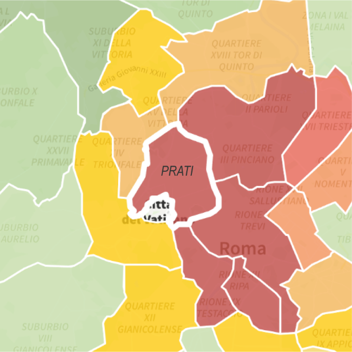
The “Prati” area represents a specific submarket within the broader urban context of the city of Rome, characterized by homogeneous extrinsic factors such as urban centrality, consolidated infrastructure, high historical and architectural value, and a stable socio-economic profile. These external characteristics contribute to defining a relatively uniform market environment, thereby ensuring that the observed differences in property values can be primarily attributed to intrinsic variables.
The case study is based on a sample of five apartments, all situated within a homogeneous area in terms of quality and availability of essential services. Each property features an elevator, comprises at least five rooms, and falls within the same building category, specifically multi-story condominiums. Notably, only non-homogeneous property characteristics have been observed among the sampled units, as detailed in Table 2.
| Unit selling price and characteristics | A | B | C | D | E |
|---|---|---|---|---|---|
| P [€/m2] | 6,312.06 | 6,533.33 | 4,600.00 | 6,428.57 | 7,500.00 |
| F. Lev. [n°] | 2 | 5 | 1 | 3 | 2 |
| Bath [n°] | 2 | 2 | 1 | 1 | 3 |
| Maint [Score] | 1 | 1 | 1 | 2 | 2 |
– Unit selling price (P), in Euros per square meter of floor area of the recently traded property.
– Floor Level (F. lev): Represented as an ordinal categorical variable ranging from the first to the fifth floor.
– Number of Bathrooms (Bath): This variable indicates the actual count of bathroom facilities present in the residence, categorized similarly to the floor levels.
– Condition of preservation and maintenance (Maint): This qualitative variable is classified into three categories with a summary evaluation: “Good/Usable” (Score “1”), “Very good/Refurbished” (Score “2”), and “Excellent/New” (Score “3”).
Other property factors that exhibit uniformity across all sampled units have been excluded from the analysis.
Table 2 presents the collected data for the sample case, while Table 3 summarizes the key descriptive statistics. The average sale price for the sample is 6,275 €/m2. The mean number of floors is 2.6. Only one property (B) in the sample features three bathrooms. Among the analyzed properties, three are classified as usable, two have been refurbished, and none are newly constructed.
| Index | Mean | Std. Error | Median | Std. Deviation | Asimm. | Min | Max |
|---|---|---|---|---|---|---|---|
| P [€/m2] | 6,274.79 | 468.93 | 6,428.57 | 1,048.56 | -1.03 | 4,600.00 | 7,500.00 |
| F. Lev. [n°] | 2.60 | 0.68 | 2.00 | 1.52 | 1.12 | 1.00 | 5.00 |
| Bath [n°] | 1.80 | 0.37 | 2.00 | 0.84 | 0.51 | 1.00 | 3.00 |
| Maint [Score] | 1.40 | 0.24 | 1.00 | 0.55 | 0.61 | 1.00 | 2.00 |
In accordance with the data presented in Table 2, the SGA has been employed for each property within the sample under analysis. In this phase, each property has been individually evaluated, with other properties treated as comparables, following the methodological principles of the SGA. The application of the SGA is not merely concerned with determining the overall market value of the subject property (see Table 4), this approach also allows for the determination of implicit prices associated with the relevant property factors, which serve as the foundation for the comparative analysis. The results on these implicit prices are presented in Table 5.
| Subject | Estimated Values [€] | Divergence between estimated values and detected prices SGA [%] |
|
|---|---|---|---|
| SGA | Selling prices | ||
| A | 5,601.59 | 6,312.06 | 11.26 |
| B | 9,841.08 | 6,533.33 | 32.62 |
| C | 5,665.70 | 4,600.00 | 23.17 |
| D | 4,297.16 | 6,428.57 | 33.16 |
| E | 9,631.42 | 7,500.00 | 28.42 |
| Implicit prices | A | B | C | D | E |
|---|---|---|---|---|---|
| F. Lev [€/n°] | 310.58 | 784.23 | 73.76 | 73.76 | 73.76 |
| Bath [€/n°] | 691.01 | 927.83 | 572.59 | 1,638,30 | 1,638.30 |
| Maint. [€/Score] | 1,207.41 | 260.11 | 615.35 | -450.35 | 1,681.06 |
From Table 4, it can be observed that the application of the SGA reveals significant discrepancies between the estimated values and the actual sale prices. The estimated value for Comparable A (5,601.59 €/m²) underestimates the sale price (6,312.06 €/m²) by 11.26%. The greatest divergence is observed for Comparable D, with a discrepancy of 33.16%, reflecting a substantially lower estimate compared to the effective price. Furthermore, notable discrepancies are evident in the case of Comparables B, C, and E, with deviations that are respectively equal to 32.62%, 23.17% and 28.42%. These findings suggest that the SGA method tends to either overestimate or underestimate the actual market values significantly.
Table 5 shows that the implicit prices for the floor level (F. Lev) are identical for Comparables C, D, and E (73.76 €/m²), whereas similar values are noted for the number of bathrooms (Bath) in Comparables D and E (1,638.30 €/m²). This uniformity points out limited empirical evidence of the SGA model in differentiating the effects of these factors, indicating potential distortions in the estimates of implicit contributions. The negative implicit price associated with the maintenance condition for Comparable D (-450.35 €/m²) is particularly noteworthy, an intuitive result that suggests a negative perception of maintenance improvements. This anomaly may arise from adverse interactions among characteristics or limitations of the model in accurately capturing the value of qualitative improvements, highlighting a potential bias in the SGA evaluations.
The implementation of the OWASM begins with an initial phase that involves evaluating empirical constraints, specifically concerning the anticipated signs of the implicit prices associated with the selected influencing factors. Considering widely acknowledged empirical phenomena, the algorithm outlined incorporates the following empirical constraints, Equation (26):
(26)
Table 6 presents the results of the market value estimations for each property in the data sample. The outputs generated by the OWASM have been compared with the actual selling prices. The OWASM demonstrates a superior alignment with actual sale prices compared to the SGA, exhibiting generally smaller discrepancies. For Comparable A, the estimated value (5,677.21 €/m²) deviates by 10.06% from the actual price, while the lowest discrepancy is observed for Comparable D (0.33%), indicating an excellent predictive capability of the method in this instance. Other discrepancies remain modest, with Comparable B showing a minimal deviation of 0.91%, and Comparables C and E exhibiting deviations of 26.98% and 9.89%, respectively.
| Subject | Estimated Values [€] | Divergence between estimated values and detected prices OWASM [%] |
|
|---|---|---|---|
| OWASM | Selling prices | ||
| A | 5,677.21 | 6,312.06 | 10.06 |
| B | 6,473.63 | 6,533.33 | 0.91 |
| C | 5,840.88 | 4,600.00 | 26.98 |
| D | 6,407.53 | 6,428.57 | 0.33 |
| E | 6,758.12 | 7,500.00 | 9.89 |
Table 7 presents the implicit prices of various features for each subject property in the data sample, derived through the implementation of the OWASM. The resulting outputs enhance the empirical reliability of the developed model. Regarding the floor level factor, the implicit price is less than €100 for only two (Properties B and E) of the five properties in the sample. These varying values could be reasonably attributed to specific market conditions and property characteristics that deviate from typical market behaviour. For example, factors such as frequent elevator malfunctions, excessive sunlight exposure on upper floors, inadequate thermal insulation on top floors, or the absence of balconies in upper levels may all contribute to this discrepancy. The bathroom factor is associated with an implicit price exceeding 200 € for four properties in the data sample (Properties B, C, D, and E), whereas it has a relatively minor influence on the valuation of Property E, with an implicit price of only 62.98 €. The condition of preservation and maintenance factor holds a substantial implicit price for Property A, amounting to 974.35 €/m2, highlighting the property’s need for renovation.
| Implicit prices | A | B | C | D | E |
|---|---|---|---|---|---|
| F. Lev [€] | 394.56 | 76.67 | 165.72 | 115.83 | 87.00 |
| Bath [€] | 62.98 | 385.68 | 267.99 | 363.26 | 229.85 |
| Maint [€] | 974.35 | 471.56 | 322.74 | 406.04 | 306.62 |
5.5. Application of the MAXENT
All computations have been carried out using MATLAB software version 9.0.0 (The MathWorks Inc.). For each subject, both the solution and the optimal value of the objective function have been calculated, along with the corresponding weights for each optimal solution (see Table 8, Table 9, Table 10, Table 11, Table 12). Generally, to derive the predicted probabilities for a particular observation, the optimal weights obtained through the optimization process can be applied to the prediction function, ensuring accurate estimations. It is essential to emphasise that the present analysis has concentrated exclusively on the characteristics of “Maint” and “F. lev.” This focus is a consequence of the MAXENT method, which further constrains the number of explanatory variables by reducing them to (m-2), where m is the total number of comparables. Consequently, only the most influential factors are retained.
| Comparable | Optimal Solution | Comparable Sale Price [€] | Contribution to the Estimated Value [€] |
|---|---|---|---|
| B | 0.1875 | 6,533.00 | 1,224.94 |
| C | 0.3125 | 4,600.00 | 1,437.50 |
| D | 0.5000 | 6,428.00 | 3,214.00 |
| E | 0.0000 | 7,500.00 | 0.00 |
| Estimated Value for Comparable [€] | 5,876.44 | ||
| Sale price detected for Comparable A [€] | 6,312.00 | ||
| % of divergence between sale price detected and estimated value for Comparable A [%] | 6.90 | ||
| Comparable | Optimal Solution | Comparable Sale Price [€] | Contribution to the Estimated Value [€] |
|---|---|---|---|
| A | 0.0000 | 6,312.00 | 0.00 |
| C | 0.5000 | 4,600.00 | 2,300.00 |
| D | 0.5000 | 6,428.00 | 3,214.00 |
| E | 0.0000 | 7,500.00 | 0.00 |
| Estimated Value for Comparable [€] | 5,514.00 | ||
| Sale price detected for Comparable B [€] | 6,533.00 | ||
| % of divergence between sale price detected and estimated value for Comparable B [%] | 15.60 | ||
| Comparable | Optimal Solution | Comparable Sale Price [€] | Contribution to the Estimated Value [€] |
|---|---|---|---|
| A | 0.3333 | 6,312.00 | 2,103.79 |
| B | 0.1667 | 6,533.00 | 1,089.05 |
| D | 0.5000 | 6,428.00 | 3,214.00 |
| E | 0.0000 | 7,500.00 | 0.00 |
| Estimated Value for Comparable [€] | 6,406.84 | ||
| Sale price detected for Comparable C [€] | 4,600.00 | ||
| % of divergence between sale price detected and estimated value for Comparable C [%] | 39.28 | ||
| Comparable | Optimal Solution | Comparable Sale Price [€] | Contribution to the Estimated Value [€] |
|---|---|---|---|
| A | 0.0000 | 6,312.00 | 0.00 |
| B | 0.3125 | 6,533.00 | 2,041.56 |
| C | 0.4375 | 4,600.00 | 2,012.50 |
| E | 0.2500 | 7,500.00 | 1,875.00 |
| Estimated Value for Comparable [€] | 5,929.06 | ||
| Sale price detected for Comparable D [€] | 6,428.57 | ||
| % of divergence between sale price detected and estimated value for Comparable D [%] | 7.77 | ||
| Comparable | Optimal Solution | Comparable Sale Price [€] | Contribution to the Estimated Value [€] |
|---|---|---|---|
| A | 0.0000 | 6,312.00 | 0.00 |
| B | 0.3125 | 6,533.00 | 2,041.56 |
| C | 0.4375 | 4,600.00 | 2,012.50 |
| D | 0.2500 | 6,428.00 | 1,607.00 |
| Estimated Value for Comparable [€] | 5,661.06 | ||
| Sale price detected for Comparable E [€] | 7,500.00 | ||
| % of divergence between sale price detected and estimated value for Comparable E [%] | 24.52 | ||
The MAXENT method exhibits significant variability in the estimated sale values, with discrepancies ranging from 6.90% to 39.28%. The most accurate result is observed for Comparable A, where the estimate (5,876.44 €/m²) deviates by only 6.90% from the actual price, demonstrating strong predictive capability in this instance. However, for Comparables C and E, the MAXENT considerably overestimates market values, with deviations of 39.28% and 24.5%, respectively. For Comparable D, the discrepancy is moderate at 7.77%, while Comparable B shows an underestimation of 15.60%. These results suggest that, despite some discrepancies, the MAXENT provides a relatively strong performance compared to the SGA and OWAS methods.
A comparison of the three methods (SGA, OWASM, and MAXENT) reveals some discrepancies in their predictive capabilities relative to observed market prices. Table 13 summarizes the results obtained in terms of market values estimated for each property in the sample. The results of the OWASM and the MAXENT have been compared with the original sales prices, and the same comparison has been reported for the SGA. Due to the heterogeneity of the sample analyzed, the SGA method has generated outputs characterized by the highest average error, equal to 25.72%. The MAXENT application has provided more accurate estimates than the SGA, the divergences between detected prices and estimated values vary between 6.9% (Comparable A) and 39.3% (Comparable C), with an average prediction error equal to 18.81%. For the considered case study, the OWASM has demonstrated the best performance overall, with an average error of 9.63%, a maximum error of 26.98% (Comparable C), and a minimum error of about 0.3% (Comparable D).
| Sub. | Comp. | Sale price detected [€/m2] | SGA | OWASM | MAXENT | |||||||
|---|---|---|---|---|---|---|---|---|---|---|---|---|
| Estimated value [€] | Divergence [%] | Estimated value [€] | Divergence [%] | Estimated value [€] | Divergence [%] | |||||||
| A | B-C-D-E | 6,312.06 | 5,601.59 | 11.26 | 5,677.21 | 10.06 | 5,876.44 | 6.90 | ||||
| B | A-C-D-E | 6,533.33 | 9,841.08 | 32.62 | 6,473.63 | 0.91 | 5,514.00 | 15.60 | ||||
| C | A-B-D-E | 4,600.00 | 5,665.70 | 23.17 | 5,840.88 | 26.98 | 6,406.84 | 39.28 | ||||
| D | A-B-C-E | 6,428.57 | 4,297.16 | 33.16 | 6,407.53 | 0.33 | 5,929.06 | 7.77 | ||||
| E | A-B-C-D | 7,500.00 | 9,631.42 | 28.42 | 6,758.12 | 9.89 | 5,661.06 | 24.52 | ||||
| Mean absolute error [%] | 25.72 | 9.63 | 18.81 | |||||||||
| Explanatory factors needed (for comparable m) | m-1 | m-1 | m-2 | |||||||||
| Implicit prices assessment | Yes | Yes | No | |||||||||
| F. Lev | Bath | Maint | F. Lev | Bath | Maint | |||||||
| A | 311 € | 691 € | 1,207 € | 395 € | 63 € | 974 € | ||||||
| B | 784 € | 928 € | 260 € | 77 € | 386 € | 472 € | ||||||
| C | 74 € | 573 € | 615 € | 166 € | 268 € | 323 € | ||||||
| D | 74 € | 1,638 € | -450 € | 116 € | 363 € | 406 € | ||||||
| E | 74 € | 1,638 € | 1,681 € | 87 € | 230 € | 307 € | ||||||
Looking more closely at the individual subjects, it is evident that for Comparable A the MAXENT is the most efficient method, with a deviation of 6.90%, compared to 11.26% for SGA, which ranks lowest in terms of performance. For Comparable B, the most accurate estimation is provided by the OWASM, with a minimal divergence of 0.91%; once again, the SGA performs worst, with a deviation of 32.62%. Interestingly, for Comparable C – where the SGA had thus far underperformed – it yields the most accurate estimate, with a deviation of 23.17%, followed by the OWASM with a very close percentage (26.98%) and the MAXENT (39.28%). In the case of Comparable D, the OWASM again achieves the best result, with an error of just 0.33%, whereas the SGA registers the poorest performance, with a 33.16% deviation. For Comparable E, the OWASM proves once more to be the most reliable, with a deviation of 9.89%, while the SGA continues to underperform, reaching a divergence of 28.48%.
Furthermore, the possibility to endogenously evaluate the implicit prices of the explanatory factors with a high empirical reliability constitutes another relevant advantage of the OWASM. This allows for the avoidance of subjectivity in determining the weights of the selected variables by the appraiser and can achieve accurate results using a limited set of comparable data. Although the implicit prices assessment represents an output of the SGA too, this method is characterized by a considerable instability in the resolution of the equation system in the presence of potential anomalies/outliers, which has a direct impact on the estimation of the implicit prices of the property characteristics being compared. On the other hand, the MAXENT does not allow inferring implicit prices of the property factors but it demonstrates considerable stability from a computational perspective.
Finally, it should be highlighted that, for the implementation of each method considered, named m the total number of comparables, the SGA and the OWASM need m-1 explanatory factors, whereas the MAXENT reduces the number of explanatory factors (m-2), in order to achieve a more streamlined and focused model. Furthermore, it should be pointed out that all three methods are not subject to operational limitations in the presence of qualitative variables too.
The economic and financial developments of recent years have significantly driven the revision of real estate valuation theories and techniques. Both in academia, where new approaches to value creation have emerged, and in practice, often characterized by ambiguity and approximation, the limitations of traditional methods have become evident. It is not uncommon for two expert appraisers to produce divergent market values for the same property, raising concerns about the precision and reliability of valuations. As a result, the accuracy of real estate valuations has become a critical priority for market participants, investors, and professionals, particularly in contexts where real estate data are scarce, and markets are opaque. In such scenarios, the collection of limited real estate data samples necessitates the optimal selection of comparable properties, as this choice significantly impacts the accuracy of the valuation. Furthermore, the increasing complexity of the factors influencing property values asks for more advanced approach methods that combine scientific rigor with user-friendliness, even for less experienced users. In this context, the present research examines the potentialities and the limits of three market approach methods, in order to provide for an improvement of the assessment reliability of professional valuers’ reports, overcoming the limitations of traditional methods in the adjustments considered for the implicit prices, and addressing the challenges associated with the use of econometric techniques in contexts characterized by a high market dynamicity. In particular, as the SGA is often applied in practice, the OWASM and the MAXENT represent two innovative methods that occupy a middle ground between traditional property evaluation techniques and advanced statistical tools, exemplified by the most modern econometric methods.
Among the three methods analyzed, for the specific case study, the OWASM and the MAXENT have shown a high statistical performance (outlined by the reduced discrepancy between estimated and observed prices). Furthermore, the assessment of the implicit prices of the explanatory factors, provided by the OWASM, has pointed out the empirical reliability of the obtained outputs. Therefore, the proposed methods (in particular, the OWASM and the MAXENT) can constitute an integration to the canonical market-oriented methods for ordinary properties (e.g. residential units, offices, shops, etc.) and income approach methods, as the Discounted Cash Flow Analysis generally applied for special properties (e.g. hotels, nursing homes, cinemas, retail spaces, etc.), so as to provide additional tools to verify the results obtained.
Further insights will concern the comparison of the methods applied in other territorial contexts, by considering different intended uses and verifying their effectiveness in the presence of limited data or highly heterogeneous property factors. Furthermore, methodological refinement may be achieved through the integration of spatial econometric components and/or machine learning tools, with the objective of enhancing model adaptability and generalisation. Another promising direction involves the development of user-friendly software interfaces to facilitate the operational use of the methods OWASM and MAXENT, thus bridging the gap between methodological innovation and daily professional application.
The paper is to be attributed in equal parts to the authors.
Agenzia del Territorio (2011) Manuale Operativo Delle Stime Immobiliari - Agenzia Del Territorio. Milano, Franco Angeli. Available at: https://www.hoepli.it/libro/manuale-operativo-delle-stime-immobiliari/9788856836745.html (Accessed 27 August 2024).
Anselin, L., & Getis, A. (1992). Spatial statistical analysis and geographic information systems. The Annals of Regional Science, 26(1), 19–33. https://doi.org/10.1007/BF01581478
Arcuri, N., De Ruggiero, M., Salvo, F., & Zinno, R. (2020). Automated valuation methods through the cost approach in a BIM and GIS integration framework for smart city appraisals. Sustainability, 12(18), 7546. https://doi.org/10.3390/su12187546
Aronsohn, A. (2020). Dealing with valuation uncertainty at times of market unrest. Available at: ire.kyiv.ua (Accessed 10 September 2024).
Associazione Bancaria Italiana (2024). Linee guida per la valutazione degli immobili in garanzia delle esposizioni creditizie. Available at: https://www.abi.it/ (Accessed 25 September 2024).
Berto, R., Stival, C. A., & Rosato, P. (2020). An integrated procedure for ex-ante evaluations of refurbishment costs in healthcare facilities. Sustainability, 12(18), 7387. https://doi.org/10.3390/su12187387
Borst, R. A. (1991). Artificial neural networks: the next modeling/calibration technology for the assessment community?’. Property Tax Journal, 10, 69–94.
Borst, R. A., & McCluskey, W. J. (2008). The modified comparable sales method as the basis for a property tax valuations system and its relationship and comparison to spatially autoregressive valuation models. In Kauko, T,. & d’Amato, M. (Eds.). Mass appraisal methods: an international perspective for property valuers. Hoboken, John Wiley & Sons, pp. 49–69. https://doi.org/10.1002/9781444301021.ch3
Bourassa, S. C., Cantoni, E., & Hoesli, M. (2007). Spatial dependence, housing submarkets, and house price prediction. The Journal of Real Estate Finance and Economics, 35(2), 143–160. https://doi.org/10.1007/s11146-007-9036-8
Brown, R. J. (2017). Entropy – what kind of bet is real estate – really? Journal of Property Investment & Finance, 35(3), 341–351. https://doi.org/10.1108/JPIF-10-2016-0078
Case, B., Clapp, J., Dubin, R., & Rodriguez, M. (2004). Modeling spatial and temporal house price patterns: a comparison of four models. The Journal of Real Estate Finance and Economics, 29(2), 167–191. https://doi.org/10.1023/B:REAL.0000035309.60607.53.
Chen, Y., Cai, Y., & Zheng, C. (2020). Efficiency of Chinese real estate market based on complexity-entropy binary causal plane method. Complexity, 2020(1), 2791352. https://doi.org/10.1155/2020/2791352
Chi Man Hui, E., Muk Fai Lau, O., & Kak Keung Lo, T. (2009). Deciphering real estate investment decisions through fuzzy logic systems. Property Management, 27(3), 163–177. https://doi.org/10.1108/02637470910964651
Ciuna, M., De Ruggiero, M., Manganelli, B., Salvo, F., & Simonotti, M. (2017). Automated valuation methods in atypical real estate markets using the mono-parametric approach. In Gervasi, O., Murgante, B., Misra, S., Borruso, G., Torre, C. M., Rocha, A. M. A. C., Taniar, D., Apduhan, B. O., Stankova, E., & Cuzzocrea, A. (Eds). Computational Science and Its Applications – ICCSA 2017. Lecture Notes in Computer Science(), vol 10406. Cham, Springer International Publishing, pp. 200–209. https://doi.org/10.1007/978-3-319-62398-6_14
Colwell, P. F., Cannaday, R. E., & Wu, C. (1983). The analytical foundations of adjustment grid methods. Real Estate Economics, 11(1), 11–29. https://doi.org/10.1111/1540-6229.00277
Copiello, S., Cecchinato, F., & Salih, M. H. (2021). The effect of hybrid attributes on property prices. Real Estate Management and Valuation, 29(4), 36–52. https://doi.org/10.2478/remav-2021-0028
Curto, R. A. (2005). L’uso delle tecniche multicriteri come procedimenti pluriparametrici. In Roscelli, R. (Ed.). Misurare nell’incertezza. Valutazioni e trasformazioni territoriali. Torino, CELID. 91–108.
De Paola, P. (2024). real estate valuations with small dataset: a novel method based on the maximum entropy principle and lagrange multipliers. Real Estate, 1(1), 26–40. https://doi.org/10.3390/realestate1010003
Domian, D., Wolf, R., & Yang, H. F. (2015). An assessment of the risk and return of residential real estate. Managerial Finance, 41(6), 591–599. https://doi.org/10.1108/MF-07-2013-0195
Festa, M. (2021). Data mining e Machine learning: la nuova frontiera dei Big data nel settore immobiliare. Territorio Italia 2021, 65–87. https://doi.org/10.14609/Ti_1_21_3i
Forte, C., & Rossi, B. D. (1979). Principi di economia ed estimo. Seconda edizione. Milano, Rizzoli.
French, N., & Gabrielli, L. (2004). The uncertainty of valuation. Journal of Property Investment & Finance, 22(6), 484–500. https://doi.org/10.1108/14635780410569470
Gabrielli, L., & French, N. (2021). Pricing to market: property valuation methods – a practical review. Journal of Property Investment & Finance, 39(5), 464–480. https://doi.org/10.1108/JPIF-09-2020-0101
Gau, G.W., Lai, T. Y., & Wang, K. (1992). Optimal comparable selection and weighting in real property valuation: an extension. Real Estate Economics, 20(1), 107–123. https://doi.org/10.1111/1540-6229.00574
Gau, G.W., Lai, T. Y., & Wang, K. (1994). A further discussion of optimal comparable selection and weighting, and a response to green. Real Estate Economics, 22(4), 655–663.
Glumac, B., & Rosiers, F. D. (2020). Practice briefing – Automated valuation models (AVMs): their role, their advantages and their limitations. Journal of Property Investment & Finance, 39(5), 481–491.
Goodman, A. C., & Thibodeau, T. (2003). Housing market segmentation and hedonic prediction accuracy. Journal of Housing Economics, 12(3), 181–201.
Iovine, R. (2015). Metodologie statistiche per la stima immobiliare. Padova, EXEO Edizioni.
Isakson, H. (2002). The linear algebra of the sales comparison approach. Journal of Real Estate Research, 24(2), 117–128. https://doi.org/10.1080/10835547.2002.12091090
Isakson, H. R. (1986). The nearest neighbors appraisal technique: an alternative to the adjustment grid methods. Real Estate Economics, 14(2), 274–286. https://doi.org/10.1111/1540-6229.00387
Isakson, H. R. (1988). Valuation Analysis of commercial real estate using the nearest neighbors appraisal technique. Growth and Change, 19(2), 11–24. https://doi.org/10.1111/j.1468-2257.1988.tb00466.x
IVSC (2021). International valuation standards: Effective 31 January 2022. London, International Valuation Standards Council.
Jaynes, E. T. (1957). Information theory and statistical mechanics. Physical Review, 106(4), 620–630. https://doi.org/10.1103/PhysRev.106.620
Kang, H. B., & Reichert, A. K. (1991). An empirical analysis of hedonic regression and grid-adjustment techniques in real estate appraisal. Real Estate Economics, 19(1), 70–91. https://doi.org/10.1111/1540-6229.00541
Kroll (2024) Ieri, Oggi, Domani. Sentiment sul Mercato Immobiliare Italiano. Available at: https://www.kroll.com/it-it/-/media/kroll-images/pdfs/ieri-oggi-domani-sentiment-sul-mercato-immobiliare-italiano-2024.pdf (Accessed 13 September 2024).
LaCour-Little, M., & Green, R. K. (1998). Are minorities or minority neighborhoods more likely to get low appraisals?’. The Journal of Real Estate Finance and Economics, 16(3), 301–315. https://doi.org/10.1023/A:1007727716513.
Lin, T., & Chang, H. (2012). How do appraisers absorb market information in property valuation? Some experimental evidence. Property Management, 30(2), 190–206. https://doi.org/10.1108/02637471211213424
Lipscomb, J., & Gray, B. (1990). An empirical investigation of four market-derived adjustment methods. Journal of Real Estate Research, 5(1), 53–66. https://doi.org/10.1080/10835547.1990.12090602
Morano, P., Tajani, F., & Locurcio, M. (2018). Multicriteria analysis and genetic algorithms for mass appraisals in the Italian property market. International Journal of Housing Markets and Analysis, 11(2), 229–262. https://doi.org/10.1108/IJHMA-04-2017-0034
Organismo Italiano di Valutazione (2015). Principi italiani di valutazione. Milano, Egea.
Özdilek, Ü. (2023). The role of thermodynamic and informational entropy in improving real estate valuation methods. Entropy, 25(6), 907. https://doi.org/10.3390/e25060907
Pace, K. (1998). Total grid estimation. Journal of Real Estate Research, 15(1), 101–114. https://doi.org/10.1080/10835547.1998.12090914
Pace, R. K., & Gilley, O. W. (1998). Generalizing the OLS and grid estimators. Real Estate Economics, 26(2), 331–347. https://doi.org/10.1111/1540-6229.00748
Pagourtzi, E., Assimakopoulos, V., Hatzichristos, T., & French, N. (2003). Real estate appraisal: a review of valuation methods. Journal of Property Investment & Finance, 21(4), 383–401. https://doi.org/10.1108/14635780310483656
Piccolo, D., & Vitale, C. (1984). Metodi statistici per l’analisi economica. Statistica e modelli lineari. 2° edizione. Bologna, Il Mulino.
Roscelli, R. (2014) Manuale di estimo. Valutazioni economiche ed esercizio della professione. Milano, UTET Università.
Rossini, P. (2000). Improving the Results of Artificial Neural Network Models for Residential Valuation. In Fourth Annual Pacific-Rim Real Estate Society Conference, Perth, Western Australia (pp. 19-21).
Ruggiero, M. D., and Salvo, F. (2011). Misure di similarità negli adjustment grid methods. Aestimum, 58, 47–58. https://doi.org/10.13128/Aestimum-9561
Shannon, C. E. (1948). A mathematical theory of communication. Bell System Technical Journal, 27(3), 379–423. https://doi.org/10.1002/j.1538-7305.1948.tb01338.x
Simonotti, M. (2006). Metodi di stima immobiliare - Applicazione degli standard internazionali. Palermo, Dario Flaccovio Editore.
Simonotti, M., Salvo, F., Ciuna, M., & De Ruggiero, M. (2016). Measurements of rationality for a scientific approach to the market-oriented methods. Journal of Real Estate Literature, 24(2), 403–427. https://doi.org/10.1080/10835547.2016.12090435
Sun, Y. (2019). Real estate evaluation model based on genetic algorithm optimized neural network. Data Science Journal, 18, 36. https://doi.org/10.5334/dsj-2019-036
Tajani, F., Morano, P., Locurcio, M., & D’Addabbo, N. (2015). Property valuations in times of crisis: artificial neural networks and evolutionary algorithms in comparison. In Gervasi, O., Murgante, B., Misra, S., Borruso, G., Torre, C. M., Rocha, A. M. A. C., Taniar, D., Apduhan, B. O., Stankova, E., & Cuzzocrea, A. (Eds). Computational Science and Its Applications – ICCSA 2017. Lecture Notes in Computer Science(), vol 10406. Cham, Springer International Publishing, pp. 194–209. Available at: https://doi.org/10.1007/978-3-319-21470-2_14
Tajani, F., Morano, P., Locurcio, M., & Torre, C.M. (2016). Data-driven techniques for mass appraisals. Applications to the residential market of the city of Bari (Italy). International Journal of Business Intelligence and Data Mining, 11(2), 109–129. https://doi.org/10.1504/IJBIDM.2016.081604
Tajani, F., Morano, P., Salvo, F., & De Ruggiero, M. (2020). Property valuation: the market approach optimised by a weighted appraisal model. Journal of Property Investment & Finance, 38(5), 399–418. https://doi.org/10.1108/JPIF-07-2019-0094
Tajani, F., & Morano, P. (2018). An empirical-deductive model for the assessment of the mortgage lending value of properties as securities for credit exposures. Journal of European Real Estate Research, 11(1), 44–70. https://doi.org/10.1108/JERER-01-2017-0007
Tecnoborsa (2018). Codice delle valutazioni immobiliari 2018 - Italian property valuation standard. Roma, Tecnoborsa SCpA.
Todora, J., & Whiterell, D. (2002). Automating the sales comparison approach. Assessment Journal, 9(1), 25–33.
Vandell, K. D. (1991). Optimal comparable selection and weighting in real property valuation. Real Estate Economics, 19(2), 213–239. https://doi.org/10.1111/1540-6229.00550
Yalpir, S., Özkan, G., & Tezel, G. (2006). The investigation of usability of artificial neural networks in the determination of residential real-estate prices. The Association for Modeling and Simulation in Enterprises AMSE, Turkey.