The stigma effect in the Land of Fires: the impact of negative environmental externalities on residential property values
1 Department of Industrial Engineering, University of Naples Federico II, Naples, Italy
2 Department of Architecture and Design, Sapienza University of Rome, Rome, Italy
*Corresponding author
E-mail: pierfrancesco.depaola@unina.it; orazio.campo@uniroma1.it; valeriascarica1994@gmail.com; marialaudando@gmail.com; liguorovalentina9@gmail.com; mario.ferraro@mail.com
Abstract. The “Land of Fires” is an area extending between the provinces of Naples and Caserta (Italy). This vast region is notoriously affected by the burial and illegal disposal of toxic and special waste in abandoned quarries or unauthorized landfills, with waste often being burned, triggering numerous toxic fires. These phenomena create a “stigma effect” on the livability of the area under examination, with the local population suffering the most significant consequences. Residents are forced to live in a territory where mortality and cancer incidence rates are significantly higher than the national average. The primary objective of this study is to assess how environmental and social quality in the “Land of Fires” influence prices in the local real estate market. The first part of the study delves into the issues of urban quality in this context and its impact on residential property prices. The second part focuses on a specific portion of the “Land of Fires”, known as the “Triangle of Death” which includes the municipalities of Acerra, Marigliano, and Nola, with the aim of evaluating the geospatial variability of real estate values.
Keywords: Land of Fires, stigma effect, environmental externalities, property values.
JEL codes: Q24, Q51, R23, R32.
Index
3. Descriptive variables of the environmental, social and urban context of the Land of Fires
3.1 Urban quality: a multidimensional character of a territory
3.3 Presence of multi-ethnic groups
3.8 Real estate market in the Land of Fires
4.1 Multiple regression models
“Contaminate” is a term etymologically derived from the Latin “taminare”, which has the precise meaning of “leaving a tactile imprint”. In its absolute sense, the term does not inherently carry either a positive or negative connotation. When applied to the history of a country, contamination can be seen as a place’s ability to welcome new peoples, thereby expanding its cultural heritage, history, and connection with the world. Through this process, it inherits new customs, traditions, and practices that endure over time, perfectly embodying the concept of “leaving a tactile imprint” inherent in the word’s etymology.
The region of Campania (Italy) has long been a land of multiple contaminations in this sense. Greeks, Romans, Spaniards, and Arabs have all been both guests and admirers of the Campanian lands, long regarded as symbols of beauty, wonder, and prosperity. The Romans even bestowed upon it the name Campania Felix, highlighting the fertility of its soil. However, today, the territorial area between the metropolitan city of Naples and the southwestern part of Caserta presents a very different image, far from an idyllic, thriving landscape.
Currently, the concept of contamination in this area carries an entirely negative meaning in the collective imagination. Human activity has left a tangible imprint, not through creation, but through the destruction of wealth and beauty. This contamination is defined by the presence of toxic substances throughout the territory, giving rise to the term “Land of Fires” (“Terra dei Fuochi” in Italian).
The expression “Land of Fires” first appeared in 2003 in the Ecomafia Report by Legambiente (2003). It was used to describe a vast geographical area encompassing 90 municipalities (56 in the province of Naples and 34 in the province of Caserta), regularly plagued by the illegal disposal and burning of toxic waste, an area covering approximately 1,076 square kilometers and home to around 2.5 million people (see Figure 1).
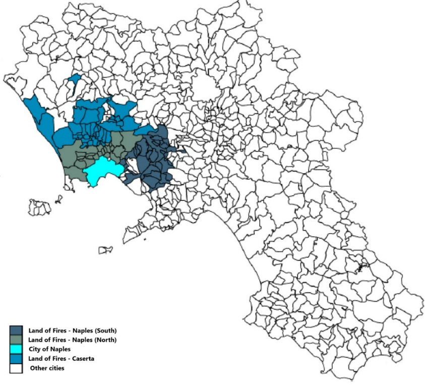
However, the term “Land of Fires” is often misused, as it originally referred specifically to the phenomenon of toxic fires and not to the burial of waste. Despite this distinction, both issues are frequently conflated under a single label.
The term “Land of Fires” has even been recognized as a neologism in the Treccani Dictionary, which defines it as: “A vast area, originally rural but now heavily urbanized, located between Naples and Caserta, characterized by frequent fires set by Camorra clans to illegally dumped toxic waste, leading to the release of highly harmful and polluting substances into the air. The situation in the northern area of Naples, which Roberto Saviano has dubbed the ‘Land of Fires’ due to the recurring waste fires that illuminate a landscape devastated by neglect, is even more dramatic. (Antonio Castaldo, Corriere della Sera, July 25, 2009, p. 11). For years, along with others, I have been recounting the disasters of the Land of Fires, which over time has swallowed up entire municipalities, constantly expanding its boundaries. Ever since Peppe Ruggiero of Legambiente coined this evocative phrase – so far removed from the Land of Fire described by Magellan – it has evoked the same image: just as the Portuguese explorer saw fires along the coast from the sea, those traveling along the Strada Statale 7 bis Terra di Lavoro (Nola-Villa Literno) or the Asse Mediano, if they take their eyes off the road, will see smoke rising from the ground, and if they lower their car windows, they will inhale a pungent, throat-burning odor with an acidic aftertaste. (Roberto Saviano, Repubblica.it, November 25, 2013, Cronaca)” (Vocabolario Treccani, 2013).
Waste management has long been at the center of political, social, economic, and health debates across the Campania region, largely due to a lack of transparency and difficulties in effectively tracing the recycling process, particularly for industrial waste. However, the “Land of Fires” is not just a snapshot of waste mismanagement specific to Campania; it can be considered a broader Italian phenomenon. Across abandoned quarries, illegal landfills, and roadside waste dumps, the same system of circumventing regulations plays out, amounting to a true ecological catastrophe.
This issue has existed for decades. According to Legambiente, between 1991 and 2013, approximately 10 million tons of various types of waste were illegally dumped in Campania (Legambiente, 2013). This included:
–slag from aluminium thermal metallurgy;
–dust from smoke purification systems;
–industrial wastewater sludge;
–liquid effluents contaminated with heavy metals;
–asbestos-containing waste;
–paint residues;
–contaminated soil from remediation activities.
The fires, on the other hand, predominantly involve urban waste, plastics, leather scraps, and textile remnants, producing devastating consequences. These include not only soil and groundwater contamination through leachate but also the release of dioxins into the air and soil. Recent regulations have been introduced to facilitate land mapping in order to assess the presence of contaminants and micro-pollutants such as polycyclic aromatic hydrocarbons (PAHs), pesticides, and heavy metals.
A 2019 study (Veritas), conducted by the Sbarro Institute for Cancer Research and Molecular Medicine at Temple University of Philadelphia, along with the National Cancer Institute – Fondazione Giovanni Pascale (Chamber of Deputies of the Italian Republic, 2022), found abnormally high levels of heavy metals in cancer patients from several municipalities in the Naples metropolitan area (Giugliano in Campania, Qualiano, Castel Volturno, and the Pianura district of Naples). Given these alarming conditions, the “medical record” of the land, water, and air in this area paints a bleak picture, where any hope for a greener, healthier future seems to decay alongside the very “monnezza” (a Neapolitan dialect term for “waste”) that represents gold for organized crime but a death sentence for the local population.
In 2025 the European Court of Human Rights has issued a final ruling condemning Italy for failing to adequately protect the inhabitants of the Land of Fires. According to the Court, the health of the population has been put at risk due to the failure to adopt effective measures to counter the phenomenon. Italy is therefore required to introduce, without delay, general measures to adequately address the pollution in the area. This is a historic ruling that acknowledges the serious institutional responsibilities in managing the environmental crisis in the Land of Fires (Corriere della Sera, 2025).
Following an analysis of the relevant literature on the “stigma effect” in the real estate market, this study first provides a territorial overview of the “Land of Fires”, highlighting its characteristics and critical issues. It then addresses the challenge of selecting appropriate indicators to measure the phenomenon and evaluate the urban quality of the region in quantitative terms. The first part of the study presents data analysis and a discussion of the results. The second part focuses on a specific area within the “Land of Fires”, known as the “Triangle of Death”, comprising the municipalities of Acerra, Marigliano, and Nola. The goal is to assess the geospatial variability of real estate values using innovative models such as Evolutionary Polynomial Regression and Geo-Additive Models.
Addressing the issue of the impacts of environmental stigma on real estate properties might initially seem to revolve around a single question: What is its economic impact on housing prices? Table 1 provides a general summary of the main references related to this issue. However, reducing the study to the resolution of a single question could lead to the misconception that the only relevant factor is the price of homes affected by contamination, disregarding other related aspects and issues.
| Year | Author(s) | Site | Issue |
|---|---|---|---|
| 1995 | Kiel K. A. | Hazardous waste sites | Impact of hazardous waste discovery, effects of disclosure of discovery announcement, influence on property values of future contaminated site cleanup |
| 1999 | Dale L., Murdoch J. C., Thayer M. A., Waddell P. A. | Lead smelter | Impacts on property values before, during and after site remediation |
| 2003 | McCluskey J. J., Rausser G. C. | Unspecified | Analysis of the short-term and long-term impact of the stigma effect |
| 2005 | Decker C. S., Nielsen D. A., Sindt R. P. | Unspecified | Impact of polluting emissions and toxic substances |
| 2006 | Simons R. A., Saginor J. D. | Unspecified | Meta-analysis of the effect of environmental contamination |
| 2007 | Kiel K. A., Williams M. | Superfund | Impact of superfund sites on local property values |
| 2008 | Neupane A., Gustavson K. | Contaminated sites | Impacts of contaminated sites |
| 2016 | Phanaeuf D. J., Liu X. | Unspecified | Stigma measurement post site cleanup |
| 2017 | Sullivan K. A. | Urban brownfield sites | Effects of remediation on property values and tax revenues |
| 2018 | Silaeva P., Akhmedinova K., Redina M., Khaustov A. | Urban areas | Evaluating the correlation between real estate prices and pollution conditions |
| 2019 | Noh Y. | Abandoned railways | Real estate market analysis before and after abandoned railways are converted into greenways |
| 2020 | Del Giudice V., De Paola P., Bevilacqua P., Pino A., Del Giudice F. P. | Abandoned industrial areas | Impacts of contaminated sites on real estate value |
| 2021 | Otsuka N., Abè H., Isehara Y., Miyagawa T. | Contaminated sites | Role of green infrastructure in brownfield regeneration |
| 2022 | Tureckovà K., Martinat S., Nevima J., Varadzin F. | Contaminated sites | Impact of distance between properties and contaminated sites |
| 2022 | Drenning P., Chowdhury S., Volchko Y., Rosén L., Andersson-Sköld Y., Norrman J. | Urban brownfield sites | Improving ecosystem services in urban brownfield sites |
The issues addressed by the scientific community are numerous, highlighting how the approach to the problem is not uniform, as it is highly dependent on the context. Soil pollution is one of the key factors contributing to the stigma effect associated with a territory, and its impact on the real estate market is particularly evident. The mere presence of contaminated land increases the perception of risk among residents and potential buyers.
The literature on this topic is extensive; however, it can generally be divided into two main areas:
–soil pollution caused by waste disposal;
–soil pollution caused by water contamination.
When thinking about soil pollution, it is most often associated with the presence of hazardous toxic waste which, through natural degradation or improper disposal processes, leads to the contamination of the surrounding land. This environmental and economic issue has been analyzed by considering the studies summarized in Table 2.
| Year | Author(s) | Causes of contamination | Objective of the study |
|---|---|---|---|
| 1992 | Ketkar K. | Hazardous waste | Impact on property values due to the presence of a hazardous landfill |
| 2004 | Ready R., Abdalla C. | Dump | Effects on property values with respect to the Euclidean distance from the site at risk |
| 2004 | Ihlanfeldt K. R., Taylor L. O. | Hazardous waste site | Effects of non-severely polluting hazardous waste sites |
| 2004 | Deaton B. J., Hoehn J.J . | Unspecified | Effects on property values with respect to the Euclidean distance from the site at risk |
| 2007 | Van Herwijnen R., Laverye T., Poole J., Hodson M. E., Hutchings T. R. | Lead | Remediation using organic materials |
| 2008 | Greenstone M., Gallagher J. | Unspecified | Comparison of landfill sites |
| 2010 | Affuso E., De Parisot C. V., Ho C. S., Hite D. | Lead | Investigation into the effect of lead pollution |
| 2011 | Braden J. B., Feng X., Won D. | Unspecified | Effects of waste polluted sites |
| 2013 | Gamper Rabindran S., Timmins C. | Hazardous waste | Localization of the benefits arising from the remediation of contaminated sites |
| 2019 | Mei Y., Gao L., Zhang P. | Dump | Relationship between landfills and residential construction prices |
| 2019 | Zwickle A. et. al. | Dioxins | Investigation into the effect of dioxin pollution |
| 2020 | Baragano D. R., Gallego J. L., Forjan R. | Heavy metals | Use of phytoremediation plants as possible toxicological indicators |
| 2023 | Shen X., Ge M., Handel S. N., Jin Z., Kirkwood N. G. | Chemical pollutants | Using spontaneous invasive plants to implement soil phytoremediation |
The analysis clearly highlights how the real estate market reflects the distrust people have in living in polluted areas, regardless of the type of contamination affecting habitat quality.
However, an environment with pollution levels exceeding the standard, once remediated and restored to acceptable ecological conditions, tends to shift perceptions regarding its suitability as a residential area, leading to a more or less significant increase in property prices.
3. Descriptive variables of the environmental, social and urban context of the Land of Fires
3.1 Urban quality: a multidimensional character of a territory
Urban quality depends on numerous factors and is primarily linked to how users perceive the territory in which they live, based on the presence or absence of any source of pollution, the development of social networks, the natural and cultural habitat, and the potential for economic growth. Considering this general perspective, we can understand that urban quality can be defined as the ability of the urban environment’s configuration to meet, both quantitatively and qualitatively, the overall material and immaterial needs of its users by providing the required services.
From this, it follows that urban quality has a multidimensional character: it is not only related to urban development but also to environmental enhancement, health protection, and the ability to satisfy social needs. In this sense, the relationship between a city’s urban quality and the needs of its users can be seen as an interaction between the demand for livability, safety, and efficiency – emanating from the local community – and the city’s ability to meet these demands. In summary, we can define urban quality based on its components (Saaty and De Paola, 2017; Del Giudice et Al., 2014):
–Environmental Quality: Dependent on the presence of specific environmental resources (climate, landscape, physical-structural characteristics of both settled and natural environments), related to both anthropic and natural systems.
–Social Quality: Dependent on socio-economic and cultural factors, often referred to as “quality of life,” including the social and cultural system, identities, and housing characteristics.
–Quality of Life: Linked to individuals’ living conditions, as reflected in the health status of the communities themselves.
Based on a meta-analysis of the literature (Sica et Al., 2025), a series of indicators have been defined for the study of urban quality (Table 3). Among these, the indicators selected for the territorial context of interest take into account that data on crime phenomena are not available at the municipal level. Moreover, the data obtained to describe land use characteristics are not correlated with temporal factors, while variables related to land consumption show limited flexibility.
| Environmental Quality | Social Quality | Quality of Life |
|---|---|---|
| Presence of dioxin | Presence of multi-ethnic groups | Cancer incidence rate |
| Presence of heavy metals and/or toxic substances | Crime rate | Respiratory disease rate |
| Presence of nearby landfills | Population density | Mortality rate |
| Recycling rate | Residential turnover rate | |
| Presence of polluted watercourses | Vacancy rate of housing units | |
| Air quality | Accessibility to essential public services | |
| Drinking water quality | Obsolescence of housing units | |
| Remediation rate (completed or planned) | ||
| Environmental certifications | ||
| Presence of abandoned industrial areas | ||
| Presence of contaminated sites | ||
| Presence of contaminated sites | ||
| Amount of waste produced | ||
| Surface area of land suitable for agricultural activities | ||
| Risk of environmental or natural disasters |
About the social environment, it is important not only to consider the presence of recorded crimes but also to take into account the coexistence of multi-ethnic communities within a given urban context. The Land of Fires, even from this perspective, presents a dramatic reality. On one hand, the high presence of immigrants might suggest a phenomenon of great inclusion and tolerance; on the other hand, it is closely linked to severe instances of labor exploitation and beyond.
In light of this consideration, it was deemed important to study the presence of foreign nationals in the Land of Fires area. For the assessment of environmental quality, however, it was considered useful to analyze the presence of landfills, as they represent a distinctive feature of this region, which suffers from ongoing illegal waste trafficking and disposal. This latter phenomenon gives rise to another critical issue: that of toxic fires. The presence of these fires turns the environment into a true incubator of pollution, affecting both air and soil with dramatic consequences for human health and the surrounding ecosystem.
It is therefore logical to assume that excluding this variable as a descriptive indicator of the reality in Land of Fires would lead to an incomplete analysis of the urban quality of the territory. Consequently, aware that the indicator accounting for the presence of toxic fires is entirely innovative compared to the long list of traditional indicators developed thus far, it was decided to include it in the analysis as it is absolutely necessary for a comprehensive and truthful description of the urban context.
Therefore, the indicators actually employed, expressed in terms of percentage variation – alongside changes in real estate prices – are as follows:
–Mortality rate;
–Presence of multi-ethnic groups;
–Rate of land reclamation;
–Presence of landfills;
–Number of toxic fires;
–Land consumption;
The indicators selected to describe the urban quality of the area under study take into account the following situations:
–available data on crime presence is not recorded at the municipal level in any public archive but only at the provincial level;
–available data related to land use does not account for temporal changes;
–land consumption represents an indicator with limited flexibility.
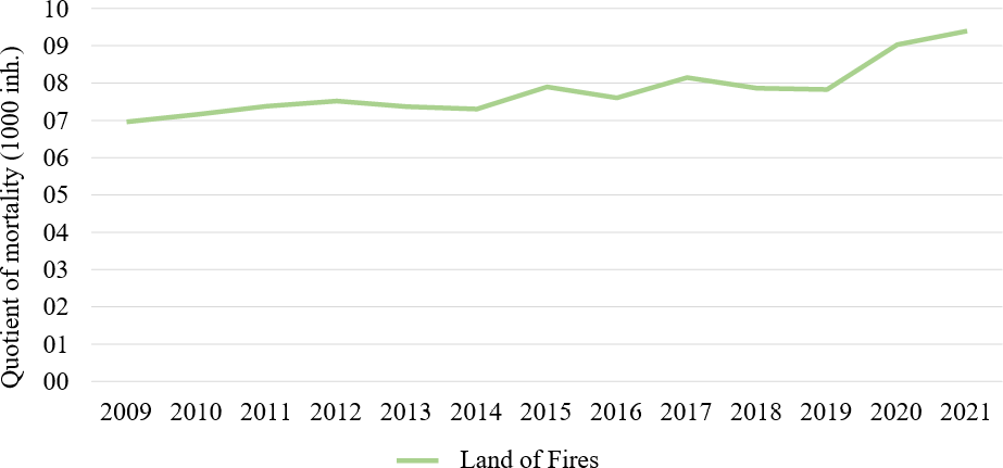
With reference to this indicator, data relating to the mortality rate of 61 municipalities of the Land of Fires were collected, for a time range that starts from 2009 and arrives at 2021 (see Appendix 1). Figure 2 summarizes the mortality quotient of the territory under investigation, obtained through an average operation of the quotients collected for each municipality and repeating the procedure for the period 2009-2021: it is possible to note a significant increase in the mortality rate over time, in reference to the entire area, taking into account the marginal contribution of all the municipalities. The mortality quotients concerning Italy and Campania and those concerning Campania and the two provinces of Naples and Caserta were also compared, where in both cases the trend is substantially similar. In the period considered, it is noted that the mortality rate in Campania is higher than the national average, while the mortality rate in Campania is lower than that of the two provinces investigated (ISTAT, 2024).
3.3 Presence of multi-ethnic groups
A key component to consider in the investigation of a crime-ridden area, useful for assessing the perception of the safety of the place, would be the crime rate, understood as the number of crimes reported in the municipalities of interest. On the one hand, the data available on crime rates are limited only to provincial levels, on the other hand, in the considered area the variable closest to the crime rate is that relating to the presence of multi-ethnic groups in the area, as a symbol not only of inclusion and acceptance but also of significant exploitation, of all kinds.
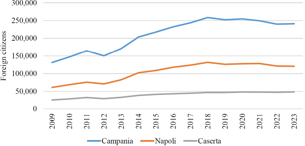
Settlement development is the driving force behind the settlement of foreign residents in the most disadvantaged places, whose attractiveness derives both from economic reasons and from poor control of the territory; in general, it is precisely the complexity in finding work in disadvantaged areas that facilitates, in addition to social marginalization, also recruitment into criminal organizations, making the perception of the place, by the community, equal to a spoiled, unsafe and unlivable environment. This condition is strongly linked to the crime rate and the number of crimes reported to the judicial authorities.
The intense phenomenon of immigration is such that it has repercussions on economic, social, demographic and cultural aspects of society; it is weighted by evaluating the presence of foreign citizens as a variable of the social and economic intertwining of the territorial context considered, taking into account the possible weight, like the environmental condition, on the investigation conducted (Forte et al., 2018).
In the period 2009-2023, the data relating to the foreign population resident in the provinces of Naples and Caserta, show a growing trend, with some municipalities showing increases of over 80-90% in the last decade analyzed (Giugliano in Campania, Castel Volturno, Mondragone), (ISTAT, 2024; Statistiche demografiche e sociali, 2024; see Appendix 2).
In order to protect areas subject to pollution, soil remediation works are considered of fundamental importance, implemented with the aim of recovering and restoring a deeply degraded environment; to do this, once the contamination of the site has been established, it is essential to implement interventions aimed at reducing or removing the sources of contamination or, in any case, aimed at decreasing the concentrations of harmful substances to a degree that is equal to or lower than those specified by the legislation, depending on the intended use of the land.
The most widespread contaminants in the territory considered are Hydrocarbons, Heavy Metals and Solvents depending on the areas and types of industrial production (ARPAC, 2024).
In the analysis conducted, a time frame was taken as a reference that starts from 2017 and arrives at 2022, where the data relating to the years 2020 and 2021 are missing. The data are represented in terms of surface area expressed in square meters (see Appendix 3).
Since we are investigating an environmental fabric characterized by strong territorial pollution, it is of fundamental importance to evaluate the presence of negative factors that constitute the pillars of the place, as they designate its peculiar characteristics; among these, the presence of landfills stands out, of a generally abusive nature in the territorial context of interest and at the basis of the contamination of the soil (by percolation into the aquifer), of the air (emissions of vapors and greenhouse gases) and of the general health of the inhabitants. Through the Regional Reclamation Plan of Campania, including a specific census of landfills – including municipal and consortium ones, both public and private – “Vast Areas” have been identified, with the aim of monitoring those surfaces within which the investigations conducted have brought to light a situation that is generally damaged and prejudiced (Regione Campania, 2024).
Briefly summarizing, using a line graph, the distribution of landfills in the territory enclosed in the Land of Fires, the following municipalities stand out from the others (see Figure 4):
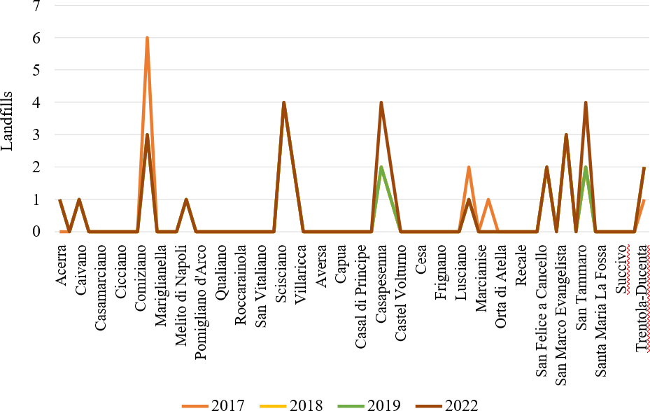
–2017: Giugliano in Campania, Marcianise, Orta di Atella and Villa Literno;
–2019: Caserta and Santa Maria La Fossa;
–2022: Giugliano in Campania, Tufino, Caserta, San Tammaro, Santa Maria La Fossa and Villa Literno.
The phenomenon of toxic fires derives from illegal activities of systematic burning of waste present in illegal landfills in order to reduce the occupied volume to a minimum (see Appendix 4).
Most of the fires are fueled by piles of special waste (i.e. deriving from industrial activities, demolition and construction activities, commercial activities, machinery, vehicles, etc.) whose management does not follow the treatment methods prescribed by environmental regulations, but the positions taken by a deep-rooted criminal system that disregards costs and controls. These events of significant problem have led to a considerable accumulation of environmental pollutants, contained in the columns of toxic fumes released, including dioxins – highly toxic and carcinogenic substances – which initially settle on grass, soil and water, and which then end up fixing themselves in the adipose tissue of animals that have ingested contaminated food and cause significant damage, not only to the ecosystem, but also to the human health of residents.
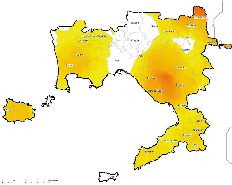
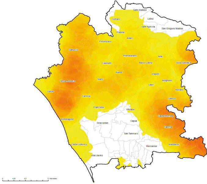
The main sources of soil pollution in Campania are gathered in the Caserta hinterland and in the territorial area located north of the province of Naples; among the contaminants, the following are mostly found: textile waste, lead and metals, acids, plastic materials, construction waste, tires and radioactive waste.
As an example, Figure 5 shows the distribution of toxic fires in the provinces of Naples (Fig. 5a) and Caserta (Fig. 5b) for year 2021 (ARPAC, 2024).
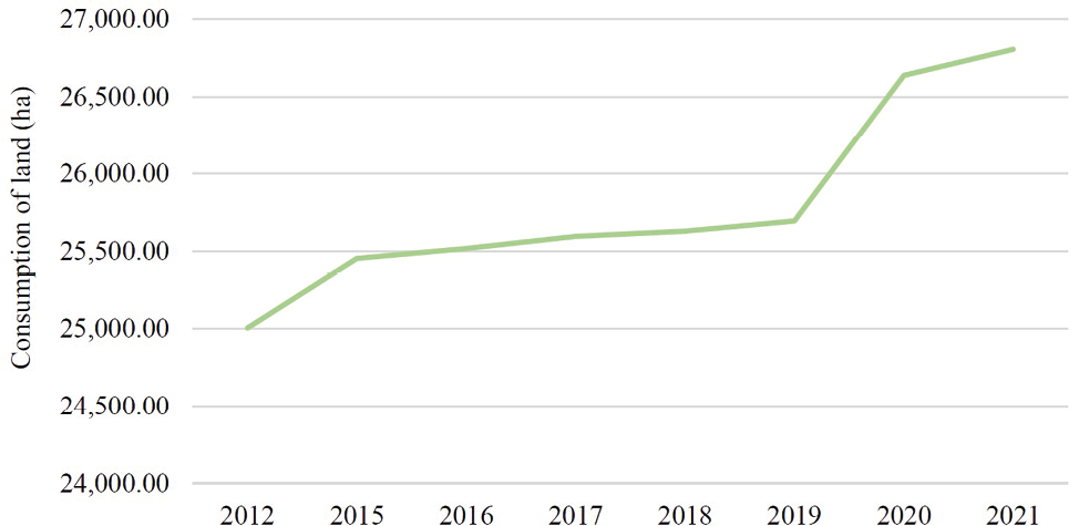
The available data consist of the surface area of consumed land (expressed in hectares), the density of land consumption in relation to the total area of each municipality (expressed in square metres/hectare), and the percentage of consumed land (see Appendices 5 and 6).
Figure 6, derived from the values in Appendix 5, show the trend of land consumption for the entire district of the Land of Fires (Sistema Nazionale per la Protezione dell’Ambiente, 2024).
3.8 Real estate market in the Land of Fires
In temporal analogy with the other indicators, the average values of the residential real estate market (€/sqm) of the municipalities constituting the Land of Fires (Immobiliare.it, 2024) were detected, in the period from 2012 to 2021 (see Appendix 7).
Through the Pareto diagram, it is quicker to identify the municipalities that present the highest trends in average annual property prices, in the time range considered. Figure 7 traces the distribution of the data collected in decreasing order and presents a cumulative line on a secondary axis as a percentage of the total.
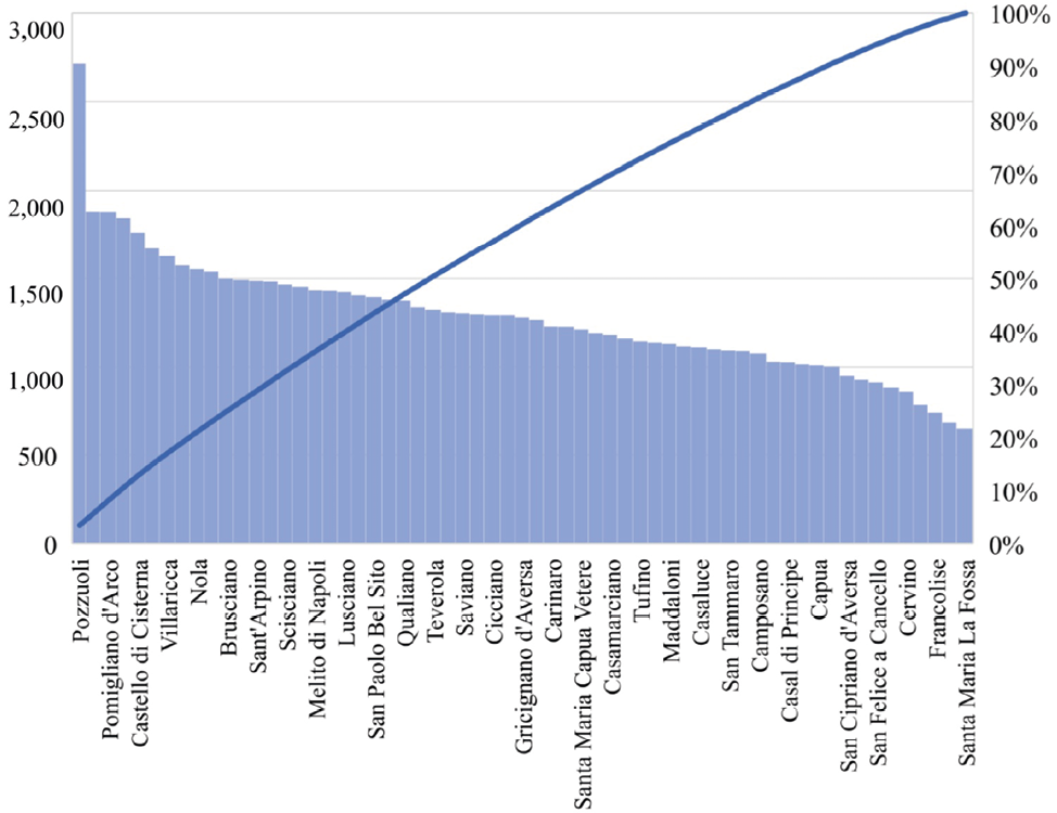
It is the municipality of Pozzuoli – followed by Quarto, Pomigliano d’Arco and Caserta – that presents the most significant values in the entire territory of the Land of Fires. Santa Maria La Fossa, Castel Volturno and Francolise are, instead, the municipalities that present the lowest trend.
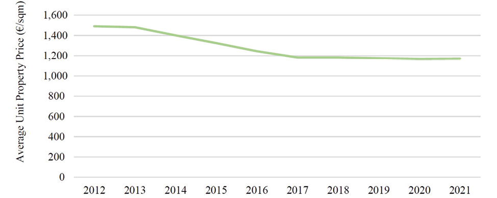
Instead, by using an average operation of the values relating to all 61 municipalities taken into consideration, the average price is obtained, discriminated for each of the years considered, of residential properties located in the Land of Fires (see Figure 8): the trend appears, in general, decreasing, with a dizzying drop after 2013 and which found substantial completion in 2017 (the year in which the recorded value was the lowest).
4.1 Multiple regression models
Multiple regression models are statistical tools used to analyze the relationship between a dependent variable (or response) and two or more independent variables (or predictors). This methodology is particularly useful for studying complex phenomena where multiple factors influence an observed outcome.
The goal is to estimate the regression coefficients that indicate the contribution of each predictor to explaining the dependent variable, while controlling for the effects of the other predictors.
The general form of the multiple linear regression model is (Simonotti, 1997):
Y = β0 + β1X1 + β2X2 + ⋯ + βpXp + ε(1)
where:
–Y: dependent variable;
–X1, X2, …, Xp: independent variables (predictors);
–β0: model intercept (expected value of Y when all X values are 0);
–β1, β2, …, βp: regression coefficients (expected change in Y for a one-unit change in Xi, holding other variables constant);
–ε: residual error (the difference between the observed and predicted values).
The coefficients βi are estimated by minimizing the sum of squared residuals (SSR), which is the difference between the observed (Yi) and predicted values.
In matrix notation, the model can be expressed as:
Y = Xβ + ε(2)
where:
–Y is the vector of observed values;
–X is the matrix of predictors;
–Β is the vector of coefficients;
–ε is the vector of errors.
The coefficients are estimated as:
= (XTX)-1XTY(3)
Main advantages of using a multiple regression model are: allows simultaneous consideration of multiple predictors, identifies relationships between variables, and provides an interpretable model. On the other hand, the main limitations are constituted by multicollinearity (when predictors are highly correlated, the estimated coefficients can become unstable), strong assumptions (requires linearity, homoscedasticity, and normality of residuals), overfitting (adding too many predictors can make the model overly complex and less generalizable).
Geoadditive models are composed by a semi-parametric additive component to express the relationship between model’s non-linear response and explanatory variables, and a component with linear mixed effects to expresses the spatial correlation of observed values (De Paola et Al., 2019 and 2021; Del Giudice et Al., 2015 and 2021).
In the case of two additive components, if (si, ti, yi), 1≤ i ≤ n, represent the measurements on two predictors s and t for the response variable y, the additive model is:
(4)
where f and g are unspecified smooth functions of s and t respectively. Therefore, if we define u+ to equal u for u > 0 and 0 otherwise, a penalized spline version of the model (4) involves the following functional form (Del Giudice & De Paola, 2014a and 2014b):
(5)
In equation (5) there is the penalization of the knot coefficients uks and ukt, where κ1s, …, κkss and κ1t, …, κktt are knots in the s and t directions respectively. The penalization of the uks and ukt is equivalent to treating them as random effects in a mixed model.
Setting β = (β0, βs, βt)T, u = (u1s, …, ukss, u1t, …, uktt)T, X = (1 si ti) with 1 ≤ i ≤ n, Z = (Zs|Zt), with:
Zs=[(si – κks)+]1 ≤ i ≤ n, 1 ≤ k ≤ Ks , Zt=[(ti – κkt)+]1 ≤ i ≤ n, 1 ≤ k ≤ Kt (6)
penalized least squares is equivalent to best linear unbiased prediction in the mixed model:
; ;
(7)
Model (7) is a variance components model since the covariance matrix of (uTεT)T is diagonal. The variance ratio σε2/σs2 acts as a smoothing parameter in s direction. Penalized spline additive models are based on low rank smoothers, considering that linear terms are easily incorporated into the model through the Xβ component.
At this point we can incorporate a geographical component by expressing kriging as a linear mixed model and merging it with an additive model such as model (7) to obtain a single mixed model (defined as geoadditive model).
Universal kriging model for (xi, yi), 1 ≤ i ≤ n (yi are scalar and xi represent geographical location included in R2 domain) is:
(8)
where S(x) is a stationary zero-mean stochastic process and εi are assumed to be independent zero-mean random variables with common variance σε2 and distributed independently of S. Prediction at an arbitrary location x0 is done through the following expression:
(9)
Then for a known covariance structure of S the resulting equation is:
(10)
where:
(11)
(12)
For all aspects and matters above reported, a geoadditive model can be described, substantially, as a single linear mixed model as follow:
(13)
Or in this further representation:
(14)
where:
; (15)
Once the useful data relating to the variables considered were collected, to provide a synthetic description of the phenomenon for each municipality, an average operation was chosen to take into account what happens in different years. A comparison was carried out between two types of averages by calculating the standard deviation: simple arithmetic mean (AM) and moving arithmetic mean (MAM). The best average was found to be the AM as it generates a lower standard deviation than the MAM. If the individual municipalities are compared based on the standard deviation, the MA is always better than the MS as the relative normal distribution is much more regular than the one considered as the MAM.
For each indicator, and in correspondence with each municipality, the average annual increase for the period 2012-2021 was developed (see Appendix 8).
In the case of interest, we referred to a regression model without an intercept, in order to ignore other possible variables on the average percentage variation of the price.
Any outliers were eliminated from the sample, namely: some small municipalities adjacent to large municipalities, as they may be affected by the influence of the phenomena of the adjacent municipality in addition to those of their own; some municipalities in the coastal area characterized by a strong phenomenon of irregular migration, such that the variable relating to the presence of foreigners would have had a preponderant aspect compared to the other independent variables.
Starting from the exploratory analysis of the regression model, the determination coefficient R2 is equal to 0.85, denoting an acceptable value in order to hypothesize a good adaptation of the regression plan to the observed points. The value of the corrected R2 is equal to 0.80, while the multiple R is equal to 0.92, returning an acceptable degree of relationship between observed and predicted values, and the relationship between the set of independent variables defined and the dependent variable is sufficiently adequate. The standard error, on the other hand, corresponds to 0.014: being close to zero, it guarantees that the regression model is accurate.
The confirmatory analysis of the model is the process of testing against a null hypothesis. In regression analysis, the null hypothesis consists in the absence of a linear relationship between the dependent variable and the explanatory variables. Since in our case p-value is associated with the F statistic < 0.05 we can affirm that there is an effective linear relationship between the independent variables and the dependent variable and that the model is not a mere theoretical construction: the relationships in the model actually exist and are not random, therefore there is evidence that at least one variable Xi significantly influences the price variable Y.
The equation of the regression model is the following:
∆price = – 0,392∙∆mortality–0,217∙∆multi-ethnic groups–0,090∙∆land reclamation+0,062∙∆landfills+0,00008∙∆toxic fires–0,791∙∆land consumption(16)
Using the regression coefficients and the mean value of the individual independent variables, it is possible to determine the influence of the individual “weighted” variable for the dependent variable; the information obtained from the Weighted Average Coefficient (WAC) is, in fact, more complete as an information set. To define the WAC, both the sign of the mean value inherent to the individual variable and the sign inherent to the “weight” deriving from the results of the regression model must be considered. A summary is provided in Table 4 where the impact of the single variable following a unitary change in price. However, if we consider the average of the price changes in the municipalities of the selected sample, we can see how much the single variable impacts the real average change ( price = -0.031).
| Variable | Regression coefficients |
|
WAC | WAC % | RWAC | RWAC% |
|---|---|---|---|---|---|---|
| ∆mortality | -0.392 | 0.037 | -0.0145 | -1.450% | 0.4677 | 46.77% |
| ∆multi-ethnic groups | -0.217 | 0.042 | -0.0091 | -0.911% | 0.2935 | 29.35% |
| ∆land reclamation | -0.009 | -0.002 | 0.00018 | 0.018% | -0.0058 | -0.581% |
| ∆landfills | +0.062 | -0.0125 | -0.00078 | -0.078% | 0.0252 | 2.516% |
| ∆toxic fires | +0.00008 | 2.519 | 0.00020 | 0.020% | -0.0065 | -0.645% |
| ∆land consumption | -0.791 | 0.006 | -0.00474 | -0.475% | 0.1529 | 15.29% |
We can define the RWAC (Relative Weighted Average Coefficient):
(17)
Through the RWAC it is found that an average change in real estate prices of -3.1% is correlated with a change of:
- +46,77% in mortality rate;
- +29.35% in the multi-ethnic groups;
- -0.581% in the unreclaimed land;
- +2.516% in the presence of landfills;
- -0.645% in toxic fires;
- +15.29% in land consumption.
It follows that: the mortality rate is the factor that most influences the collapse of real estate prices, followed by the rate of multi-ethnic groups and land consumption. The same qualitative information is obtained from the WAC: observing the absolute value, the ranking of the variables that affect the cost is the same.
Considering the average variation of a phenomenon has allowed us to examine phenomena of temporal evolution in a stationary manner: the results we obtained must therefore always be read in terms of variation in a “horizontal” manner.
There is an inverse relationship between the mortality rate and the variation in prices, the same one present with the rate of multi-ethnic groups, unreclaimed land and land consumption; this implies that as one of the above-mentioned rates increases, there is a decrease in the increase, over time, of real estate prices. The distrust resulting from the poor liveability of a generally unhealthy urban context, such as that of the Land of Fires, is tangible from the high values of all four of the above-mentioned variables; life in a territory that presents: a higher mortality rate than the national average (the causes of which are strongly linked to the low urban quality of the place), a high rate of multi-ethnic groups, tending to increase, generally overshadowed by the possibility of an “easy life” offered by organized crime (just think of the migrant settlements – located in unauthorized or abusive areas – that turn into a real business for eco-mafias), high levels of unreclaimed land and particularly the land consumed by artificial casings, cannot but translate into a disadvantage, which also affects property prices, in which the distrust deriving from the dangerousness of the place is poured, without remedy, onto the real estate market discouraging the value of the assets pertaining to it. However, in the analysis conducted, there are two rates that, by increasing, generate positive variations in prices, they are the presence of landfills and that of toxic fires.
Concerning the first factor, the data show that, from 2017 to 2021, there was a reduction in the quantity of active landfills in the territory, consequently generating an increase in decommissioned plants (a landfill that does not comply with European directives is a danger during the work phase as well as during closure, since the resulting leachate penetrates the subsoil causing irreparable and profound pollution); this increase, while on the one hand it may seem like a potentially positive effect and generate an increase in changes in real estate prices, in reality it hides serious negative implications. The last rate discussed is that relating to fires; the harmful fires for which we have information are those collected by official monitoring that uses actual video surveillance booths. It is a variable with a very low weight – in the order of 10-5 – whose positive influence on price changes deserves careful attention; the positive variation in the number of fires recorded is seen to correspond to a positive variation in prices, the impact of which is very small, being a phenomenon characterized by a negative prerogative and extremely monitored and opposed. Despite the actions implemented regarding monitoring, knowledge and prevention, it remains a disadvantageous factor in terms of the liveability of the place.
Synthesizing, in short, what has been exposed, it is clearly noted that the majority of environmental and social phenomena, considered in the analysis, lead to a negative variation in property prices; this is indicative of a real estate market that receives an increasingly smaller number of consents and that appears vigorously stigmatized by the indelible mark that pollution has placed on the territory (the stigma effect, in fact, is not only linked to the dangerousness of the phenomenon but also, and above all, to the perception that one has of it). The situation worsens if we consider that phenomena such as the setting of fires, dumping activities, and the presence of illegal landfills dedicated to the disposal of illicit waste, appear to be out of control, taking on a greater gravity in the eyes of those who perceive it.
Of the 61 municipalities that are part of the Land of Fires, the municipalities of Acerra, Nola and Marigliano, due to their geographical positioning and the high mortality linked to the onset of tumors, have been defined as “the triangle of death”.
The high mortality rate in these municipalities appears to be mainly linked to pollution caused by the illegal dumping of toxic substances in the environment managed by the Camorra, which operates an illegal waste traffic throughout the country, transporting industrial waste produced by industries in northern Italy to the Campania region. The illegal dumping of waste occurs in illegal landfills but often also in legal landfills, all accompanied by the phenomenon of fires that already devastate the entire area of the Land of Fires.
To describe the real estate market of this territory in spatial terms, n. 384 residential properties, chosen in such a way as to homogeneously cover the territory of the 3 municipalities, were detected during the year 2021 (Immobiliare.it, 2024). The real estate market remained stationary until 2024. To take into account the different locations, the data were “homogenized” through specific market ratios drawn up based on data from the Real Estate Market Observatory of the Italian Revenue Agency (Osservatorio del Mercato Immobiliare, Agenzia delle Entrate, 2024).
For each property the real estate market price and the amounts of some real estate characteristics are known, as shown in Table 5 and Table 6.
| UPRICE | FLOOR | MAIN | CAR | |
|---|---|---|---|---|
| Mean | 1285.08 | 1.50 | 1.31 | 1.125 |
| Standard Error | 26.26 | 0.087 | 0.047 | 0.050 |
| Median | 1237.24 | 1.00 | 1.00 | 1.00 |
| Standard Deviation | 514.65 | 1.71 | 0.91 | 0.98 |
| Sample variance | 264869.60 | 2.92 | 0.83 | 0.96 |
| Interval | 2983.33 | 10.00 | 3.00 | 7.00 |
| Variable | Description |
|---|---|
| Real estate price (PRICE) | expressed in Euro |
| Commercial surface (SUR) | expressed in sqm |
| Real estate unitary price (UPRICE) | expressed in Euro/sqm |
| Commercial surface (SUR) | expressed in sqm |
| Level of floor (FLOOR) | cardinal scale |
| Maintenance status (MAIN) | expressed via a score scale varying from 0 to 3, starting from buildings to be renovated up to new ones; |
| Number of parking spaces (CAR) | cardinal scale |
| Geographic coordinates (XCOORD, YCOORD) | expressed with longitude and latitude |
Based on real estate data, the following geoadditive model has been implemented:
UPRICE = FLOOR + MAIN + CAR + f(XCOORD, YCOORD)(18)
Results and main indices of model verification are presented in tables and graphics that follow. The determination of knots for the spatial component and its geographical coordinates are identified by the space filling algorithm, implemented in default.knots.2D function library of R Software Wand et Al., 2005). The geoadditive model was therefore estimated by the Re.M.L. method using the spm library of R software.
A preliminary multiple regression analysis conducted on the data relating to the individual municipalities, to verify the reliability of the data used in the geoadditive model, is provided in Table 7.
| Acerra (116 properties) | Marigliano (133 properties) | Nola (135 properties) | |
|---|---|---|---|
| Multiple R2 | 0.944 | 0.961 | 0.950 |
| R2 | 0.891 | 0.924 | 0.903 |
| Adjusted R2 | 0.879 | 0.915 | 0.894 |
The estimates of effects in the non-linear model have been significant by values of freedom degrees (df) and smoothing parameters (spar). The values of obtained predictions are consistent with observed data, also analysis of residuals has not shown any abnormality in its structure. In examined area, the spatial distribution of real estate unitary prices clearly shows how the geographical component affects the prices of sampled properties.
The main result of the interpolation is a thematic map depicting the real estate unitary values in the urban context considered, in which blue and red colors represent unitary values, respectively, lowest and highest values (see Figure 9).
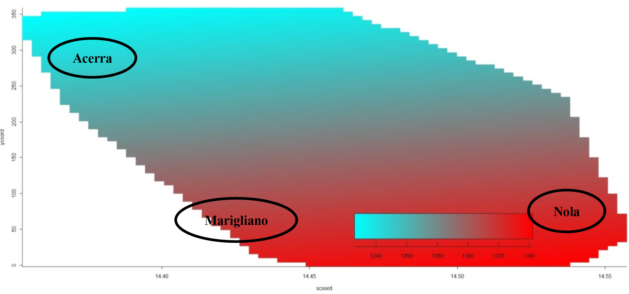
From Figure 9 it can be observed that unit prices increase from the municipality of Acerra (high vertex of the triangle, with lower prices) to that of Nola (low vertex of the triangle, with higher prices).
Unit sales prices cover a range from € 1220/sqm to € 1340/sqm and fall within the range of values provided by the Real Estate Market Observatory of the Italian Revenue Agency for the areas analysed.
The analysis of the geo-additive model appears to be in line with a series of phenomena related to the urban quality of the municipal contexts considered. To explain the phenomenon of the variability of unit prices between these three municipalities, in the municipality of Acerra there are 137 industries, in that of Marigliano 322 and in that of Nola 484: the number of industries increases from municipality to municipality and with it, the perception of the potential for growth and economic development increases and in accordance with this it is easy to think that a greater prospect of a better environment from a socio-economic point of view is linked to a greater real estate value. If we take into account the fact that in Nola there is the Campania interport, which is an international logistics platform connected to the main world hubs, we realize that the higher sale price, demonstrated by the geo-additive model, of the properties in this area is largely justified. If we consider the percentage of consumed land as an indicator of urbanization (how much artificial has been built on the territory), we see that, for increasing values of the percentage of consumed land, the municipal ranking we obtain is: Acerra, Marigliano, Nola. Therefore, Acerra appears to be the least urbanized municipality while Marigliano is the medium urbanized one while Nola is the most urbanized one. For this reason, it can be assumed that, since the price of a property is directly linked to the urban context and the services that a certain place offers, it increases with the increase in the degree of urbanization since the increase in the latter also increases the services that the city can offer to its residents. The fact that the lowest selling prices refer to the municipality of Acerra, the highest ones to the municipality of Nola and the intermediate ones to the municipality of Marigliano, can also be linked to other factors that are also linked to the perception of healthiness of the area. If we consider that moving from the municipality of Acerra to that of Nola there is a reduction in polluted surfaces of 10%, we can understand how an urban context of better environmental quality is certainly associated with a higher price of properties since environmental quality is an asset that impacts the quality of life of residents who are therefore willing to pay more to live in an urban context that is considered better as it is home to a lower polluting impact.
When talking about remediation and soil pollution, it is good to remember that the chemical, physical and biological alteration of the soil is linked to anthropic phenomena and human activities that can compromise it, even irreversibly. In this regard, it can be considered that among the most disastrous causes is the incorrect disposal of waste, which often occurs without regulations and in a completely abusive manner. The municipalities considered are part, as we know, of the broader context of the Land of Fires characterized by the presence of abusive fires that are triggered to burn waste that is sometimes even toxic and dangerous. Following this, we realize that going to live in a context where there is a greater ignition of toxic fires is certainly less inviting than going to live in places where phenomena of this type do not occur. If we move from the municipality of Nola to that of Acerra, the data on the ignition of fires (obviously we are talking about those registered but the real number is much higher as the phenomenon appears to be uncontrolled), an increase in fires, on average per year, of 60% is recorded, therefore it is easy to understand that prices in correspondence with this notable increase undergo a notable decrease as the perception, and the actual, dangerousness of the phenomenon discourages buyers from living in these areas.
This work was aimed at verifying how environmental and social externalities influence the market prices of residential buildings in the Land of Fires.
The results obtained make it clear that the problems strongly related to environmental pollution strongly influence the real estate market, even if their consequences appear, only theoretically, less worthy of consideration than those generated by the elements concerning the mortality risk and those relating to social risks, specific to the territory taken into consideration.
The clear sign of a real estate market that admits a number of consents that is gradually declining is visible in the reduction of property values in the selected municipalities, guilty of being located on a land affected by an indelible stigma, related not only to environmental pollution – due to the scattered and massive toxic fires and harmful elements discernible from abandoned industrial and waste disposal sites – but also to an ever-increasing trend in mortality (which sees the development of tumor diseases as the main cause) and multi-ethnic groups subjugated by the presence of criminal organizations, capable of actively establishing themselves in social reasoning.
Through data processing tools, it has been concluded that positional characteristics have effects on the formation of market prices, but how can this information be put to good use? Rather than implementing future estimates regarding the trend of costs, it would be of fundamental and primary importance to make changes to the sick matrix of the “Land of Fires”, not only from the point of view of environmental remediation which, only marginally, is already underway – through innovative soil phytoremediation technologies, which allow the restoration of the original conditions, replacing those physical-chemical steps that return totally infertile soils – but also by determining more precise comparison frameworks, in particular for the municipalities not included in the final analysis and through continuous monitoring of those factors that generate the greatest critical issues, drawing inspiration from the operations already implemented regarding the “fire issue”. The crisis of the Land of Fires serves as a harsh reminder of the complex interaction between industrialization, lax regulation and environmental degradation and highlights the need for proactive measures to prevent similar crises from emerging elsewhere. It is clear that by learning from the mistakes made on this soil, governments, industries and civil societies can work together to create a more sustainable future, characterised by responsible waste management, strong regulatory frameworks and a commitment to preserving the health of the planet and its inhabitants.
Affuso, E., de Parisot, C. V., Ho, C.S., & Hite, D. (2010). The impact of hazardous waste on property values: the effect of lead pollution. Urbani Izziv, 21(2), 117–126.
ARPAC – Agenzia Regionale per la Protezione Ambientale della Campania (2024). Available at: https://www.arpacampania.it (accessed 30 October 2024)
Baragaño, D., Forján, R., Welte, L., & Gallego, J. L. R. (2020). Nanoremediation of As and metals polluted soils by means of graphene oxide nanoparticles. Scientific Reports, 10(1), 1896.
Braden, J. B., Feng, X., & Won, D. (2011). Waste sites and property values: a meta-analysis. Environmental and Resource Economics, 50, 175–201.
Chamber of Deputies of the Italian Republic (2022). Meeting report of the 18.1.2022. Available at: https://www.camera.it (accessed 20 January 2025)
Corriere della Sera (2025). Terra dei Fuochi, la Cedu condanna l’Italia: mette a rischio la vita degli abitanti. Don Patriciello: “Quante calunnie subite”. Available at: https://napoli.corriere.it/notizie/cronaca/25_gennaio_30/terra-dei-fuochi-la-cedu-l-italia-mette-a-rischio-la-vita-degli-abitanti-e531ff37-353e-40bc-8287-80280f6ecxlk.shtml?refresh_ce (accessed 30 January 2025)
Dale, L., Murdoch, J. C., Thayer, M. A., & Waddell, P. A. (1999). Do property values rebound from environmental stigmas? Evidence from Dallas. Land Economics, 311–326.
Deaton J., & Hoehn J. J. (2004). Hedonic analysis of hazardous waste sites in the presence of other urban disamenities. Environmental Science & Policy, 7(6), 499–508.
Decker, C. S., Nielsen, D. A., & Sindt, R. P. (2005). Residential property values and community right‐to‐know laws: Has the toxics release inventory had an impact?. Growth and Change, 36(1), 113–133.
De Paola, P., Del Giudice, V., Massimo, D. E., Forte, F., Musolino, M., & Malerba, A (2019). Isovalore maps for the spatial analysis of real estate market: a case study for a central urban area of Reggio Calabria, Italy. In Calabrò, F., Della Spina, L., & Bevilacqua, C. (Eds.). New Metropolitan Perspectives. Smart Innovation, Systems and Technologies, Vol. 100, pp. 402-410. Cham (Switzerland), Springer. https://doi.org/10.1007/978-3-319-92099-3_46
De Paola, P., Del Giudice, V., Massimo, D. E., Del Giudice, F. P., Musolino, M., & Malerba, A (2021). Green building market premium: detection through spatial analysis of real estate values. A case study. In Bevilacqua, C., Calabrò, F., & Della Spina, L. (Eds.). New Metropolitan Perspectives. Smart Innovation, Systems and Technologies, vol 178, pp.1413- 1422. Cham (Switzerland), Springer. https://doi.org/10.1007/978-3-030-48279-4_132
Del Giudice, V., & De Paola, P. (2014a). Geoadditive models for property market. Applied Mechanics and Materials, 584, 2505–2509. https://doi.org/10.4028/www.scientific.net/AMM.584-586.2505
Del Giudice, V., & De Paola, P. (2014b). The effects of noise pollution produced by road traffic of Naples Beltway on residential real estate values. Applied Mechanics and Materials, 587, 2176–2182. https://doi.org/10.4028/www.scientific.net/amm.587-589.2176.
Del Giudice, V., De Paola, P., & Torrieri, F. (2014). An integrated choice model for the evaluation of urban sustainable renewal scenarios. Advanced Materials Research, 1030, 2399–2406. https://doi.org/10.4028/www.scientific.net/amr.1030-1032.2399
Del Giudice, V., Manganelli, B., De Paola, P. (2015). Spline Smoothing for Estimating Hedonic Housing Price Models. In Gervasi, O., Murgante, B., Misra, S., Gavrilova, M. L., Coutinho Rocha, A. M. A., Torre, C., Taniar, D., Apduhan, B. O. (Eds.). Computational Science and Its Applications -- ICCSA 2015. ICCSA 2015. Lecture Notes in Computer Science, vol 9157. Cham, Springer. https://doi.org/10.1007/978-3-319-21470-2_15
Del Giudice, V., De Paola, P., Bevilacqua, P., Pino, A., & Del Giudice, F. P. (2020). Abandoned industrial areas with critical environmental pollution: evaluation model and stigma effect. Sustainability, 12(13), 5267.
Del Giudice, V., Massimo, D. E., De Paola, P., Del Giudice, F. P., & Musolino, M. (2021). Green Buildings for post carbon city: determining market premium using spline smoothing semiparametric method. In Bevilacqua, C., Calabrò, F., & Della Spina, L. (Eds.). New Metropolitan Perspectives. Smart Innovation, Systems and Technologies, vol 178. Cham (Switzerland), Springer. https://doi.org/10.1007/978-3-030-48279-4_114
Drenning, P., Chowdhury, S., Volchko, Y., Rosén, L., Andersson-Sköld, Y., & Norrman, J. (2022). A risk management framework for Gentle Remediation Options (GRO). Science of the Total Environment, 802, 149880.
Forte, F., Antoniucci, V., & De Paola, P. (2018). Immigration and the housing market: the case of Castel Volturno, in Campania region, Italy. Sustainability, 10(2), 343. https://doi.org/10.3390/su10020343
Gamper-Rabindran, S., & Timmins, C. (2013). Does cleanup of hazardous waste sites raise housing values? Evidence of spatially localized benefits. Journal of Environmental Economics and Management, 65(3), 345–360.
Greenstone, M., & Gallagher, J. (2008). Does hazardous waste matter? Evidence from the housing market and the superfund program. The Quarterly Journal of Economics, 123(3), 951–1003.
Ihlanfeldt, K. R., & Taylor, L. O. (2004). Externality effects of small-scale hazardous waste sites: evidence from urban commercial property markets. Journal of Environmental Economics and Management, 47(1), 117–139
Immobiliare.it (2024). Available at: https://www.immobiliare.it (accessed 30 October 2024).
ISTAT (2024). Available at: https://www.istat.it (accessed 30 October 2024)
Ketkar, K. (1992) Hazardous waste sites and property values in the State of New Jersey. Applied Economics, 24(6), 647–659.
Kiel, K. A. (1995). Measuring the impact of the discovery and cleaning of identified hazardous waste sites on house values. Land Economics, 428–435.
Kiel, K. A., & Williams, M. (2007). The impact of Superfund sites on local property values: are all sites the same?. Journal of Urban Economics, 61(1), 170–192.
Legambiente (2003). Rapporto Ecomafia. Available at: www.legambiente.it (accessed 30 September 2024).
Legambiente (2013). Le rotte della Terra dei Fuochi. Available at: https://legambiente.campania.it/wp-content/uploads/2014/04/1115rotte_terradeiFuochi.pdf (accessed 30 September 2024).
McCluskey, J. J., & Rausser, G. C. (2003). Stigmatized asset value: is it temporary or long-term?. Review of Economics and Statistics, 85(2), 276–285.
Mei, Y., Gao, L., & Zhang, P. (2019). Residential property price differentials of waste plants: evidence from Beijing, China. Applied Economics, 51(55), 5952–5960.
Neupane, A., & Gustavson, K. (2008). Urban property values and contaminated sites: A hedonic analysis of Sydney, Nova Scotia. Journal of Environmental Management, 88(4), 1212–1220.
Noh, Y. (2019). Does converting abandoned railways to greenways impact neighboring housing prices? Landscape and urban planning, 183, 157–166.
Osservatorio del Mercato Immobiliare, Agenzia delle Entrate (2024). Available at: https://www.agenziaentrate.gov.it (accessed 30 October 2024).
Otsuka, N., Abe, H., Isehara, Y., & Miyagawa, T. (2021). The potential use of green infrastructure in the regeneration of brownfield sites: three case studies from Japan’s Osaka Bay Area. Local Environment, 26(11), 1346–1363.
Phaneuf, D. J., & Liu, X. (2016). Disentangling property value impacts of environmental contamination from locally undesirable land uses: implications for measuring post-cleanup stigma. Journal of Urban Economics, 93, 85–98.
Ready, R. C., & Abdalla, C. W. (2004). The impacts of land use on nearby property values: estimates from a hedonic house price model. In Bergstrom, J. C., Goetz, S. J., & Shortle, J. S. (Eds.). Land use problems and conflicts: causes, consequences and solutions. pp. 202-218. London, Routledge Taylor & Francis Group.
Regione Campania (2024). Available at: https://www.regione.campania.it (accessed 30 October 2024)
Saaty, T. L., & De Paola, P. (2017). Rethinking design and urban planning for the cities of the future. Buildings, 7(3), 76. https://doi.org/10.3390/buildings7030076
Shen, X., Ge, M., Handel, S. N., Wang, W., Jin, Z., & Kirkwood, N. G. (2023). Advancing environmental design with phytoremediation of brownfield soils using spontaneous invasive plants. Science of The Total Environment, 883, 163635.
Sica, F., De Paola, P., Tajani, F., & Doko, E. (2025). Spatial–Temporal Ontology of Indicators for Urban Landscapes. Land, 14(1), 72.
Silaeva, P., Akhmedinova, K., Redina, M., & Khaustov, A. (2018). Identification of environmental characteristics of urban areas as a factor in the formation of property prices. International Multidisciplinary Scientific GeoConference Surveying Geology and Mining Ecology Management, SGEM. International Multidisciplinary Scientific Geoconference. 2018. pp. 727-732.
Simonotti, M. (1997). La stima immobiliare. Torino, UTET Editore.
Simons, R., & Saginor, J. (2006). A meta-analysis of the effect of environmental contamination and positive amenities on residential real estate values. Journal of Real Estate Research, 28(1), 71–104.
Sistema Nazionale per la Protezione dell’Ambiente (2024). Available at: https://www.snpambiente.it (accessed 30 October 2024).
Statistiche demografiche e sociali (2024). Available at: https://www.tuttitalia.it (accessed 30 October 2024).
Sullivan, K. A. (2017). Brownfields remediation: Impact on local residential property tax revenue. Journal of Environmental Assessment Policy and Management, 19(03), 1750013.
Turečková, K., Martinát, S., Nevima, J., & Varadzin, F. (2022). The Impact of Brownfields on Residential Property Values in Post-Industrial Communities: A Study from the Eastern Part of the Czech Republic. Land, 11(6), 804.
van Herwijnen, R., Laverye, T., Poole, J., Hodson, M. E., & Hutchings, T. R. (2007). The effect of organic materials on the mobility and toxicity of metals in contaminated soils. Applied Geochemistry, 22(11), 2422–2434.
Vocabolario Treccani (2013). Neologismi 2013. Available at: https://www.treccani.it (accessed 20 January 2025).
Wand, M. P., French, J. L., Ganguli, B., Kammann, E. E., Stuadenmayer, J., & Zanobetti, A. (2005). SemiPar 1.0 R package. Available at: https://cran.r-project.org.
Zwickle, A., Cox, J. G., Zhuang, J., Hamm, J. A., Upham, B. L., Chung, M., ... & Dearing, J. W. (2019). The effect of dioxin contamination and remediation on property values. International Journal of Environmental Research and Public Health, 16(20), 3900.
| Municipalities | 2009 | 2010 | 2011 | 2012 | 2013 | 2014 | 2015 | 2016 | 2017 | 2018 | 2019 | 2020 | 2021 |
|---|---|---|---|---|---|---|---|---|---|---|---|---|---|
| Acerra | 6.5 | 6.1 | 6.1 | 6.5 | 6.7 | 6.3 | 7.1 | 7 | 6.7 | 6.7 | 7.1 | 7.9 | 8.5 |
| Brusciano | 6.5 | 7.1 | 7.2 | 6.2 | 7 | 6.6 | 7.5 | 5.9 | 7.4 | 7.5 | 6.2 | 8.5 | 9.2 |
| Caivano | 6.5 | 8.1 | 7.3 | 7.1 | 6.6 | 7 | 7.7 | 7.1 | 7.6 | 6.7 | 7.9 | 9.8 | 10.3 |
| Camposano | 8.1 | 7.9 | 9.2 | 9.4 | 9 | 8.1 | 10.5 | 10.3 | 10.7 | 9.6 | 9.9 | 11.2 | 10.6 |
| Casamarciano | 8.3 | 7.7 | 12.1 | 8.6 | 9.2 | 10.9 | 9.7 | 11 | 9.8 | 11.1 | 10.2 | 11.6 | 15.4 |
| Castello di Cisterna | 5.9 | 5.6 | 7.1 | 6.9 | 6.8 | 6.8 | 7 | 6 | 6.7 | 5.4 | 6.3 | 6.8 | 7.8 |
| Cicciano | 9.3 | 7.3 | 7.5 | 9.6 | 7.2 | 9 | 8.9 | 9.1 | 9 | 9.7 | 10.4 | 8.9 | 10.6 |
| Cimitile | 8.4 | 9.5 | 11.4 | 8.3 | 7.5 | 7 | 9.9 | 9.8 | 8.1 | 11.5 | 10.4 | 11.9 | 9.4 |
| Comiziano | 11.6 | 8.8 | 8.2 | 9.3 | 10.9 | 10.4 | 12.1 | 8.3 | 13.8 | 9.6 | 8 | 14.2 | 14.1 |
| Giugliano in Campania | 5.3 | 5.5 | 5.5 | 6.5 | 6 | 5.6 | 6.4 | 5.6 | 6.3 | 5.9 | 5.6 | 7.2 | 6.9 |
| Mariglianella | 7.2 | 7.2 | 6.8 | 6.3 | 6.2 | 5.8 | 6.7 | 7.3 | 6.7 | 6.2 | 7.3 | 8.1 | 10.28 |
| Marigliano | 8.4 | 8.5 | 7.8 | 9 | 8.6 | 8.8 | 9.2 | 8.7 | 9.6 | 9.1 | 9 | 10.1 | 10.2 |
| Melito di Napoli | 5.2 | 5.1 | 4.9 | 5.5 | 4.4 | 5.8 | 6.2 | 6 | 5.6 | 5.8 | 5.8 | 6.7 | 7.6 |
| Nola | 8.8 | 9.4 | 8.7 | 9.4 | 8.5 | 8.5 | 8.7 | 9.9 | 9.2 | 8.5 | 8.4 | 9 | 10.1 |
| Pomigliano d’Arco | 7.8 | 7.7 | 9.2 | 7.7 | 8.2 | 8.4 | 8.6 | 8.9 | 9.2 | 7.9 | 8.5 | 9.9 | 10.1 |
| Pozzuoli | 6.7 | 6.5 | 6.8 | 8.1 | 7.9 | 7.8 | 8.1 | 7.8 | 8.5 | 7.9 | 7.8 | 9.5 | 9.9 |
| Qualiano | 6.1 | 5.8 | 7 | 6 | 6.2 | 7 | 7.5 | 7.3 | 8 | 7.6 | 7.2 | 9.2 | 9.4 |
| Quarto | 6 | 5 | 5.3 | 5.7 | 5.3 | 5.4 | 7 | 6.2 | 6.2 | 5.7 | 6.5 | 6.4 | 6.9 |
| Roccarainola | 9.5 | 9.9 | 9.6 | 7 | 9.8 | 7.9 | 6.6 | 8.5 | 11.9 | 10.7 | 11.5 | 10.1 | 12.1 |
| San Paolo Bel Sito | 7.4 | 6.5 | 5.4 | 9.2 | 8.5 | 8.5 | 9.4 | 9.1 | 11.8 | 9.3 | 9.1 | 7.7 | 8.9 |
| San Vitaliano | 5.7 | 7.6 | 7.7 | 7.3 | 8.1 | 7 | 9.6 | 7.8 | 9.9 | 10.2 | 7.7 | 9.9 | 9.2 |
| Saviano | 7.9 | 7.9 | 9.6 | 8.6 | 9.1 | 7.9 | 9.2 | 7.9 | 9.8 | 7.9 | 9.6 | 11.2 | 11 |
| Scisciano | 5.6 | 8.1 | 7.1 | 8.6 | 8.5 | 8 | 8.2 | 8 | 7.1 | 6.9 | 6.5 | 8.7 | 8.5 |
| Tufino | 8.8 | 6.4 | 4.8 | 9.8 | 9.6 | 5.1 | 8.2 | 6.7 | 8.7 | 8.5 | 6.9 | 12.3 | 13.7 |
| Villaricca | 5.3 | 5.4 | 6 | 5.5 | 6.6 | 5.7 | 6.8 | 6.9 | 7.1 | 7 | 7.5 | 8.6 | 8.7 |
| Visciano | 9.8 | 10.7 | 10.1 | 9.7 | 10.9 | 10.7 | 11.2 | 8.3 | 13.3 | 11.2 | 10.8 | 13.3 | 10.7 |
| Aversa | 7.7 | 7.3 | 7.9 | 8.6 | 7.6 | 8.7 | 8.9 | 7.9 | 9 | 8.6 | 8.5 | 10.3 | 9.4 |
| Capodrise | 5.6 | 6.7 | 6 | 6.6 | 6.2 | 4.4 | 5.8 | 5.9 | 6.8 | 6.8 | 5.7 | 8.7 | 7.7 |
| Capua | 10.2 | 9.1 | 9.8 | 12.1 | 8.8 | 9.7 | 10.6 | 10.8 | 10.9 | 9.4 | 10.8 | 11.4 | 11.3 |
| Carinaro | 5.8 | 9 | 5.6 | 6.9 | 9.6 | 6.5 | 7.5 | 6.7 | 7.7 | 7.6 | 7.3 | 5.8 | 8.8 |
| Casal di Principe | 4.2 | 5.5 | 5.9 | 5.8 | 6.1 | 6.8 | 6.6 | 7 | 7.4 | 6.4 | 7 | 7.9 | 9.4 |
| Casaluce | 6.2 | 6.3 | 8 | 5.7 | 5.9 | 5.6 | 7.1 | 6.3 | 8.5 | 7.3 | 7.4 | 7.7 | 9.4 |
| Casapesenna | 3.6 | 6.2 | 6.7 | 6.3 | 6.8 | 7.7 | 7 | 5.7 | 7.9 | 8.9 | 7.3 | 11 | 11.5 |
| Caserta | 8.1 | 8.5 | 8.6 | 9.1 | 9.3 | 8.7 | 10.3 | 9.3 | 9.7 | 9.7 | 9.5 | 11.4 | 10.1 |
| Castel Volturno | 10 | 8.7 | 7.6 | 9 | 7.6 | 7.6 | 8.4 | 7.9 | 7.8 | 8 | 6.9 | 8.5 | 8.6 |
| Cervino | 8.8 | 9.7 | 7.9 | 11 | 7.3 | 8.1 | 8.3 | 8.6 | 5.6 | 7.8 | 9.2 | 9.8 | 8.3 |
| Cesa | 5 | 6.2 | 5.8 | 5 | 5 | 6.1 | 6.1 | 5.5 | 5.7 | 5.8 | 5.9 | 7.2 | 7.4 |
| Francolise | 7.2 | 9.4 | 9.5 | 10.2 | 12.4 | 11.8 | 7.7 | 11 | 9.2 | 8.9 | 9.9 | 9.1 | 10.4 |
| Frignano | 8.1 | 7.8 | 7.9 | 7.9 | 7.6 | 7.5 | 8.6 | 8.2 | 8.5 | 9.5 | 7.6 | 7.7 | 9.5 |
| Gricignano di Aversa | 4.9 | 4.1 | 4.4 | 4.8 | 4 | 4.5 | 6.1 | 4.2 | 5.6 | 5.9 | 5.7 | 7.2 | 5.1 |
| Lusciano | 5 | 6 | 6.5 | 7.3 | 6.3 | 6.4 | 7.6 | 6.7 | 5.9 | 6.6 | 5.7 | 7.4 | 6.8 |
| Maddaloni | 7.6 | 8 | 7.2 | 8 | 8.4 | 7.2 | 8 | 7.1 | 8.5 | 8.3 | 8 | 8.9 | 9.3 |
| Marcianise | 6.4 | 6.6 | 6.4 | 7.4 | 6.9 | 7.3 | 8 | 7.1 | 7.6 | 7.9 | 6.9 | 7.6 | 9.3 |
| Mondragone | 7.8 | 9.6 | 8.5 | 8.6 | 9 | 7.6 | 8.9 | 8.8 | 9.1 | 9 | 8.8 | 10.1 | 10.7 |
| Orta di Atella | 3.9 | 3.8 | 3.9 | 3.4 | 4 | 4.5 | 4.7 | 4.6 | 4.7 | 4.6 | 4.5 | 5.2 | 5.3 |
| Parete | 6.2 | 7.4 | 7 | 5.7 | 6.7 | 6.3 | 6 | 6.6 | 7.1 | 6.7 | 6.2 | 7.8 | 7.5 |
| Recale | 6.6 | 6.8 | 6.2 | 6.4 | 6.1 | 8.8 | 7 | 8.4 | 8.5 | 6 | 7.7 | 8.4 | 8.9 |
| San Cipriano d’Aversa | 4.8 | 6.1 | 8.2 | 7.3 | 7.3 | 7.1 | 9 | 9.4 | 9 | 7.5 | 8.4 | 10.6 | 11.7 |
| San Felice a Cancello | 8.2 | 7.3 | 8.8 | 7.2 | 6.4 | 8.1 | 9 | 8.8 | 9.5 | 9.9 | 8.8 | 11.2 | 10.7 |
| San Marcellino | 5.2 | 7.5 | 6.3 | 7.5 | 5.7 | 6.7 | 6.6 | 6.3 | 6.7 | 7.4 | 7.3 | 7.6 | 7 |
| San Marco Evangelista | 5.7 | 6.2 | 5.6 | 7.8 | 6.4 | 6.8 | 6.5 | 6.6 | 7 | 5.8 | 8.3 | 8.7 | 9.3 |
| San Nicola la Strada | 7.5 | 7.7 | 7.8 | 6 | 7.3 | 7.4 | 7.4 | 6.9 | 7.7 | 8.1 | 7.9 | 8.9 | 8.6 |
| San Tammaro | 4.6 | 6.9 | 7.8 | 7.2 | 6.7 | 6.3 | 4.9 | 8.3 | 9.3 | 6.7 | 8.7 | 8.2 | 9.6 |
| Santa Maria Capua Vetere | 9 | 10 | 11.3 | 10.2 | 11.1 | 10.4 | 11 | 10.1 | 9.7 | 10.7 | 9.8 | 10.9 | 10.7 |
| Santa Maria la Fossa | 9.6 | 7.7 | 9.2 | 10.1 | 8.5 | 9.5 | 15.7 | 9.6 | 7.1 | 10.5 | 9.1 | 9 | 12.5 |
| Sant’Arpino | 6.8 | 5.3 | 6.5 | 6.4 | 6.2 | 5.9 | 6.8 | 6.5 | 7.4 | 5.8 | 7.2 | 8.1 | 9.3 |
| Succivo | 7.5 | 5.3 | 6.9 | 6.1 | 6.1 | 7.3 | 6.2 | 6.6 | 7.1 | 7.7 | 6.9 | 8.3 | 6.9 |
| Teverola | 4.6 | 4.9 | 5.9 | 4.9 | 5.9 | 4.7 | 6.2 | 5.6 | 5.8 | 5.8 | 7 | 7.4 | 5.9 |
| Trentola Ducenta | 6.4 | 5.1 | 5.5 | 5.4 | 6.7 | 5.3 | 6.4 | 5 | 6.3 | 6 | 6.8 | 6.6 | 7.5 |
| Villa di Briano | 6.5 | 5.3 | 5.2 | 6.7 | 4.8 | 6.5 | 2.8 | 8.1 | 8.1 | 7.1 | 5.6 | 8.3 | 9.7 |
| Villa Literno | 6.3 | 7.4 | 7.6 | 8.3 | 5.6 | 5.9 | 6.2 | 6.5 | 5.9 | 6.7 | 7.3 | 9.1 | 9.9 |
| Municipalities | 2009 | 2010 | 2011 | 2012 | 2013 | 2014 | 2015 | 2016 | 2017 | 2018 | 2019 | 2020 | 2021 | 2022 | 2023 |
|---|---|---|---|---|---|---|---|---|---|---|---|---|---|---|---|
| Acerra | 1,231 | 1,378 | 1,133 | 1,240 | 1,756 | 1,797 | 1,830 | 1,952 | 2,092 | 2,008 | 2,192 | 2,187 | 2,128 | 2,208 | 2,294 |
| Brusciano | 199 | 227 | 215 | 221 | 270 | 290 | 324 | 310 | 296 | 287 | 279 | 275 | 257 | 237 | 208 |
| Caivano | 552 | 637 | 605 | 663 | 692 | 667 | 708 | 756 | 800 | 864 | 850 | 858 | 813 | 818 | 780 |
| Camposano | 95 | 122 | 107 | 122 | 138 | 141 | 141 | 142 | 143 | 142 | 130 | 126 | 104 | 86 | 78 |
| Casamarciano | 53 | 52 | 56 | 62 | 66 | 62 | 60 | 51 | 55 | 51 | 43 | 43 | 40 | 40 | 46 |
| Castello di Cisterna | 122 | 150 | 127 | 131 | 152 | 154 | 152 | 161 | 163 | 170 | 178 | 173 | 178 | 163 | 144 |
| Cicciano | 228 | 282 | 243 | 242 | 315 | 322 | 341 | 341 | 357 | 374 | 355 | 340 | 245 | 243 | 245 |
| Cimitile | 120 | 142 | 134 | 187 | 198 | 210 | 232 | 242 | 247 | 262 | 275 | 246 | 254 | 232 | 208 |
| Comiziano | 46 | 56 | 37 | 35 | 47 | 48 | 49 | 54 | 54 | 54 | 52 | 50 | 46 | 49 | 53 |
| Giugliano in Campania | 3,470 | 3,974 | 2,702 | 3,393 | 4,555 | 5,229 | 6,098 | 6,512 | 6,980 | 6,908 | 6,914 | 6,087 | 6,569 | 6,184 | 5,844 |
| Mariglianella | 152 | 174 | 190 | 218 | 243 | 232 | 213 | 225 | 242 | 239 | 237 | 236 | 232 | 245 | 231 |
| Marigliano | 677 | 772 | 778 | 827 | 939 | 1,032 | 1,111 | 1,112 | 1,112 | 1,144 | 1,124 | 1,097 | 1,022 | 990 | 1,021 |
| Melito di Napoli | 348 | 401 | 296 | 393 | 446 | 596 | 585 | 678 | 750 | 815 | 771 | 722 | 739 | 714 | 632 |
| Nola | 907 | 979 | 887 | 931 | 1,046 | 1,138 | 1,201 | 1,248 | 1,357 | 1,440 | 1,497 | 1,524 | 1,425 | 1,283 | 1,290 |
| Pomigliano d’Arco | 575 | 648 | 646 | 714 | 840 | 870 | 911 | 943 | 960 | 960 | 1,042 | 1,016 | 935 | 919 | 954 |
| Pozzuoli | 1,638 | 1,768 | 1,254 | 2,071 | 1,899 | 2,045 | 2,056 | 2,151 | 2,176 | 2,220 | 2,273 | 2,263 | 2,199 | 1,931 | 1,889 |
| Qualiano | 519 | 607 | 497 | 575 | 685 | 867 | 1,038 | 1,055 | 1,108 | 1,130 | 1,195 | 1,128 | 1,075 | 1,023 | 1,025 |
| Quarto | 351 | 425 | 406 | 483 | 525 | 593 | 653 | 719 | 734 | 754 | 793 | 760 | 898 | 814 | 766 |
| Roccarainola | 137 | 148 | 139 | 176 | 184 | 184 | 193 | 194 | 202 | 176 | 213 | 205 | 143 | 143 | 150 |
| San Paolo Bel Sito | 76 | 96 | 73 | 79 | 87 | 92 | 85 | 80 | 81 | 74 | 75 | 74 | 74 | 70 | 79 |
| San Vitaliano | 88 | 109 | 108 | 117 | 117 | 109 | 99 | 95 | 106 | 128 | 145 | 144 | 132 | 126 | 128 |
| Saviano | 383 | 437 | 453 | 469 | 529 | 586 | 618 | 724 | 770 | 849 | 849 | 815 | 733 | 686 | 689 |
| Scisciano | 91 | 98 | 97 | 115 | 127 | 139 | 153 | 169 | 179 | 181 | 167 | 164 | 163 | 156 | 154 |
| Tufino | 53 | 48 | 48 | 51 | 48 | 54 | 64 | 64 | 50 | 54 | 49 | 49 | 33 | 37 | 31 |
| Villaricca | 454 | 504 | 503 | 544 | 639 | 685 | 703 | 690 | 799 | 792 | 704 | 721 | 699 | 703 | 683 |
| Visciano | 129 | 111 | 111 | 111 | 113 | 103 | 101 | 98 | 77 | 76 | 89 | 88 | 84 | 83 | 81 |
| Aversa | 1,939 | 2,100 | 2,248 | 2,530 | 2,747 | 2,914 | 2,963 | 3,037 | 3,099 | 3,203 | 3,103 | 3,019 | 3,030 | 2,876 | 2,951 |
| Capodrise | 241 | 278 | 213 | 190 | 240 | 247 | 252 | 267 | 290 | 287 | 327 | 313 | 289 | 293 | 295 |
| Capua | 749 | 874 | 747 | 813 | 927 | 972 | 1,067 | 1,069 | 1,117 | 1,159 | 1,266 | 1,178 | 1,236 | 1,337 | 1,518 |
| Carinaro | 266 | 270 | 230 | 255 | 311 | 320 | 315 | 312 | 309 | 312 | 306 | 299 | 354 | 333 | 344 |
| Casal di Principe | 617 | 718 | 660 | 815 | 913 | 988 | 1,052 | 1,171 | 1,164 | 1,164 | 1,317 | 1,234 | 1,327 | 1,409 | 1,482 |
| Casaluce | 345 | 401 | 421 | 494 | 522 | 553 | 503 | 486 | 439 | 473 | 370 | 350 | 370 | 418 | 445 |
| Casapesenna | 220 | 249 | 191 | 220 | 313 | 379 | 437 | 473 | 539 | 540 | 449 | 438 | 496 | 514 | 550 |
| Caserta | 2,997 | 3,345 | 2,568 | 2,735 | 3,402 | 3,575 | 3,605 | 3,632 | 3,793 | 4,007 | 4,048 | 3,955 | 3,825 | 3,775 | 3,916 |
| Castel Volturno | 2,512 | 2,933 | 3,071 | 3,415 | 3,568 | 3,854 | 3,880 | 3,954 | 4,114 | 4,012 | 4,352 | 4,081 | 4,691 | 4,933 | 4,824 |
| Cervino | 111 | 135 | 77 | 88 | 141 | 155 | 143 | 151 | 168 | 184 | 183 | 174 | 158 | 167 | 182 |
| Cesa | 209 | 246 | 225 | 231 | 270 | 283 | 296 | 302 | 305 | 337 | 350 | 342 | 336 | 313 | 311 |
| Francolise | 182 | 224 | 201 | 216 | 243 | 266 | 280 | 300 | 305 | 289 | 296 | 282 | 292 | 288 | 348 |
| Frignano | 272 | 266 | 172 | 182 | 283 | 296 | 288 | 290 | 320 | 328 | 337 | 334 | 366 | 345 | 347 |
| Gricignano di Aversa | 403 | 461 | 384 | 431 | 513 | 388 | 484 | 522 | 544 | 599 | 870 | 853 | 881 | 806 | 807 |
| Lusciano | 362 | 431 | 457 | 578 | 577 | 655 | 656 | 705 | 730 | 772 | 793 | 779 | 719 | 734 | 764 |
| Maddaloni | 598 | 731 | 778 | 803 | 835 | 900 | 950 | 950 | 1,027 | 1,080 | 838 | 820 | 881 | 889 | 944 |
| Marcianise | 751 | 834 | 861 | 873 | 882 | 922 | 981 | 1,025 | 1,122 | 1,224 | 1,268 | 1,204 | 1,203 | 1,145 | 1,152 |
| Mondragone | 1,286 | 1,598 | 1,741 | 2,110 | 2,578 | 2,857 | 3,079 | 3,231 | 3,521 | 3,909 | 4,581 | 4,279 | 4,111 | 3,689 | 3,717 |
| Orta di Atella | 369 | 449 | 411 | 482 | 578 | 666 | 739 | 747 | 752 | 760 | 800 | 813 | 754 | 674 | 673 |
| Parete | 528 | 607 | 565 | 586 | 769 | 853 | 876 | 873 | 888 | 917 | 997 | 987 | 1,015 | 1,037 | 1,083 |
| Recale | 233 | 249 | 301 | 304 | 321 | 337 | 356 | 251 | 232 | 240 | 242 | 231 | 241 | 247 | 248 |
| San Cipriano d’Aversa | 529 | 627 | 453 | 520 | 615 | 721 | 736 | 796 | 917 | 972 | 1,034 | 1,009 | 869 | 845 | 826 |
| San Felice a Cancello | 424 | 483 | 315 | 338 | 418 | 438 | 438 | 469 | 502 | 485 | 498 | 474 | 515 | 543 | 563 |
| San Marcellino | 608 | 699 | 500 | 602 | 841 | 940 | 1,026 | 1,030 | 1,036 | 1,060 | 1,062 | 1,075 | 49 | 990 | 971 |
| San Marco Evangelista | 171 | 185 | 202 | 238 | 268 | 299 | 334 | 366 | 369 | 372 | 334 | 320 | 302 | 293 | 290 |
| San Nicola la Strada | 798 | 920 | 816 | 853 | 1,097 | 1,246 | 1,365 | 1,599 | 1,701 | 1,632 | 1,505 | 1,393 | 1,380 | 1,356 | 1,304 |
| San Tammaro | 99 | 107 | 56 | 76 | 100 | 88 | 94 | 104 | 99 | 93 | 162 | 154 | 161 | 176 | 194 |
| Santa Maria Capua Vetere | 1,198 | 1,349 | 1,068 | 1,107 | 1,403 | 1,453 | 1,478 | 1,560 | 1,739 | 1,819 | 1,729 | 1,695 | 1,729 | 1,629 | 1,692 |
| Santa Maria la Fossa | 74 | 111 | 89 | 108 | 120 | 168 | 191 | 173 | 167 | 163 | 127 | 135 | 136 | 143 | 162 |
| Sant’Arpino | 268 | 299 | 214 | 256 | 304 | 328 | 324 | 403 | 461 | 487 | 500 | 483 | 537 | 495 | 513 |
| Succivo | 179 | 226 | 200 | 242 | 278 | 300 | 336 | 341 | 322 | 365 | 369 | 371 | 407 | 371 | 338 |
| Teverola | 364 | 411 | 370 | 390 | 498 | 505 | 521 | 505 | 508 | 517 | 444 | 438 | 447 | 424 | 410 |
| Trentola Ducenta | 623 | 679 | 443 | 517 | 704 | 758 | 785 | 799 | 804 | 834 | 953 | 943 | 848 | 829 | 873 |
| Villa di Briano | 249 | 331 | 184 | 286 | 343 | 384 | 607 | 539 | 597 | 640 | 643 | 580 | 628 | 601 | 591 |
| Villa Literno | 743 | 588 | 349 | 430 | 752 | 900 | 919 | 960 | 1,085 | 1,274 | 1,336 | 1,275 | 1,214 | 1,428 | 1,572 |
| Potentially contaminated/unremediated sites | 2017 | 2018 | 2019 | 2022 |
|---|---|---|---|---|
| Acerra | 1,623,710 | 1,642,711 | 1,502,449 | 1,419,196 |
| Brusciano | 60,634 | 60,641 | 60,641 | 58,251 |
| Caivano | 1,956,060 | 1,809,272 | 1,825,433 | 1,555,704 |
| Camposano | 2,967 | 2,968 | 2,968 | 2,968 |
| Casamarciano | 254,613 | 254,624 | 254,624 | 254,624 |
| Castello di Cisterna | 161,353 | 161,361 | 161,361 | 161,361 |
| Cicciano | 47,805 | 47,806 | 47,806 | 47,806 |
| Cimitile | 15,506 | 15,511 | 15,511 | 15,511 |
| Comiziano | 204,927 | 204,930 | 204,930 | 204,930 |
| Giugliano in Campania | 6,745,723 | 6,227,107 | 6,227,107 | 6,026,963 |
| Mariglianella | 62,874 | 62,878 | 64,418 | 62,418 |
| Marigliano | 339,325 | 339,337 | 334,521 | 302,341 |
| Melito di Napoli | 109,784 | 109,791 | 109,791 | 109,791 |
| Nola | 1,516,436 | 1,517,647 | 1,510,233 | 1,423,718 |
| Pomigliano d’Arco | 2,969,546 | 2,764,587 | 2,753,607 | 2,779,028 |
| Pozzuoli | 1,136,506 | 1,755,157 | 1,647,277 | 1,646,228 |
| Qualiano | 126,601 | 126,604 | 126,604 | 126,604 |
| Quarto | 247,859 | 247,864 | 231,268 | 247,864 |
| Roccarainola | 194,532 | 194,535 | 194,535 | 194,535 |
| San Paolo Belsito | 838 | 839 | 839 | 839 |
| San Vitaliano | 202,069 | 202,074 | 183,030 | 182,439 |
| Saviano | 133,842 | 133,846 | 133,846 | 133,846 |
| Scisciano | 37,860 | 37,863 | 37,863 | 37,863 |
| Tufino | 534,917 | 534,925 | 534,925 | 534,925 |
| Villaricca | 284,988 | 285,251 | 285,251 | 285,251 |
| Visciano | 0 | 0 | 0 | 0 |
| Aversa | 96,603 | 99,238 | 84,238 | 83,548 |
| Capodrise | 68,047 | 68,050 | 42,838 | 40,976 |
| Capua | 2,463,009 | 2,468,933 | 2,460,209 | 2,308,087 |
| Carinaro | 174,472 | 182,170 | 182,170 | 182,170 |
| Casal di Principe | 36,988 | 41,091 | 37,991 | 36,700 |
| Casaluce | 22,593 | 22,594 | 22,594 | 20,660 |
| Casapesenna | 2,523 | 2,523 | 2,523 | 2,523 |
| Caserta | 1,246,361 | 1,239,682 | 1,627,890 | 1,535,614 |
| Castel Volturno | 3,973,000 | 3,982,183 | 3,982,183 | 3,972,524 |
| Cervino | 27,112 | 27,115 | 27,115 | 27,115 |
| Cesa | 8,805 | 9,266 | 9,266 | 6,807 |
| Francolise | 172,385 | 172,393 | 172,393 | 172,393 |
| Frignano | 58,542 | 58,545 | 58,545 | 58,545 |
| Gricignano d’Aversa | 179,818 | 179,820 | 179,820 | 179,820 |
| Lusciano | 3,907 | 3,907 | 3,907 | 3,907 |
| Maddaloni | 1,463,828 | 1,400,585 | 1,357,122 | 1,360,644 |
| Marcianise | 853,513 | 850,915 | 783,752 | 806,145 |
| Mondragone | 1,121,746 | 1,120,669 | 1,118,795 | 1,115,339 |
| Orta di Atella | 296,016 | 281,053 | 281,053 | 281,053 |
| Parete | 16,617 | 16,617 | 16,617 | 16,617 |
| Recale | 21,901 | 21,902 | 21,902 | 21,902 |
| San Cipriano d’Aversa | 1,187 | 1,187 | 1,187 | 1,187 |
| San Felice a Cancello | 237,554 | 237,565 | 237,565 | 237,565 |
| San Marcellino | 2,193 | 2,194 | 2,194 | 2,194 |
| San Marco Evangelista | 410,870 | 410,891 | 410,891 | 410,891 |
| San Nicola La Strada | 160,081 | 160,085 | 160,085 | 160,085 |
| San Tammaro | 703,837 | 703,849 | 703,849 | 703,849 |
| Santa Maria Capua Vetere | 400,209 | 396,163 | 381,641 | 381,641 |
| Santa Maria La Fossa | 417,560 | 405,642 | 405,642 | 405,643 |
| Sant’Arpino | 234 | 234 | 234 | 234 |
| Succivo | 48,360 | 48,361 | 48,361 | 48,361 |
| Teverola | 491,270 | 493,267 | 492,115 | 485,715 |
| Trentola-Ducenta | 57,710 | 57,712 | 57,712 | 57,712 |
| Villa di Briano | 119,787 | 119,790 | 119,790 | 119,790 |
| Villa Literno | 1,514,918 | 1,514,921 | 1,514,921 | 1,514,920 |
| Municipalities | 2014 | 2015 | 2016 | 2017 | 2018 | 2019 | 2020 | 2021 |
| Acerra | 5 | 8 | 5 | 3 | 47.26 | 81.79 | 73.28 | 53.29 |
| Caivano | 4 | 19 | 4 | 11 | 85.72 | 148.02 | 132.61 | 94.43 |
| Castello di Cisterna | 0 | 2 | 0 | 0 | 4.5 | 7.79 | 6.98 | 5.08 |
| Giugliano in Campania | 2 | 96 | 65 | 27 | 472.61 | 740.09 | 663.05 | 482.14 |
| Marigliano | 0 | 1 | 0 | 0 | 2.25 | 3.89 | 3.49 | 2.54 |
| Melito di Napoli | 0 | 0 | 0 | 1 | 2.25 | 3.89 | 3.49 | 2.54 |
| Pozzuoli | 0 | 10 | 1 | 2 | 29.26 | 50.64 | 45.37 | 32.99 |
| San Vitaliano | 0 | 0 | 0 | 0 | 0 | 0 | 0 | 0 |
| Qualiano | 0 | 12 | 9 | 6 | 60.76 | 105.17 | 94.22 | 68.51 |
| Aversa | 0 | 0 | 2 | 1 | 3.11 | 3.49 | 3.48 | 1.99 |
| Capua | 0 | 1 | 0 | 1 | 2.07 | 2.32 | 2.32 | 1.33 |
| Carinaro | 0 | 0 | 1 | 1 | 2.07 | 2.32 | 2.32 | 1.33 |
| Casal di Principe | 4 | 6 | 1 | 1 | 12.44 | 13.94 | 13.91 | 7.98 |
| Casaluce | 0 | 1 | 0 | 1 | 2.07 | 2.32 | 2.32 | 1.33 |
| Castel Volturno | 0 | 4 | 23 | 3 | 31.09 | 34.85 | 34.78 | 19.95 |
| Frignano | 0 | 2 | 2 | 2 | 6.22 | 6.97 | 6.96 | 3.99 |
| Gricignano d’Aversa | 0 | 3 | 2 | 3 | 8.29 | 9.29 | 9.27 | 5.32 |
| Lusciano | 0 | 1 | 0 | 0 | 1.04 | 1.16 | 1.16 | 0.66 |
| Maddaloni | 0 | 0 | 1 | 1 | 2.07 | 2.32 | 2.32 | 1.33 |
| Marcianise | 0 | 0 | 0 | 0 | 0 | 0 | 0 | 0 |
| Mondragone | 0 | 0 | 17 | 1 | 18.66 | 20.91 | 20.87 | 11.97 |
| Orta di Atella | 0 | 2 | 0 | 0 | 2.07 | 2.32 | 2.32 | 1.33 |
| Parete | 0 | 1 | 0 | 0 | 1.04 | 1.16 | 1.16 | 0.66 |
| San Cipriano d’Aversa | 0 | 1 | 0 | 1 | 2.07 | 2.32 | 2.32 | 1.33 |
| San Felice a Cancello | 0 | 0 | 0 | 0 | 0 | 0 | 0 | 0 |
| San Marco Evangelista | 0 | 0 | 0 | 0 | 0 | 0 | 0 | 0 |
| San Tammaro | 0 | 10 | 1 | 0 | 11.4 | 12.78 | 12.75 | 7.32 |
| Santa Maria Capua Vetere | 0 | 6 | 0 | 0 | 6.22 | 6.97 | 6.96 | 3.99 |
| Succivo | 0 | 2 | 0 | 1 | 3.11 | 3.49 | 3.48 | 1.99 |
| Teverola | 0 | 3 | 2 | 2 | 7.26 | 8.13 | 8.12 | 4.66 |
| Trentola Ducenta | 0 | 1 | 2 | 0 | 3.11 | 3.49 | 3.48 | 1.99 |
| Villa Literno | 0 | 5 | 11 | 6 | 22.8 | 25.56 | 25.51 | 14.63 |
| Villa di Briano | 0 | 0 | 2 | 1 | 3.11 | 3.48 | 3.48 | 1.99 |
| Municipalities | 2012 | 2015 | 2016 | 2017 | 2018 | 2019 | 2020 | 2021 |
|---|---|---|---|---|---|---|---|---|
| Acerra | 1.040.27 | 1.049.54 | 1.050.65 | 1.053.00 | 1.053.67 | 1.058.77 | 1.158.86 | 1.179.91 |
| Brusciano | 202.33 | 202.55 | 202.69 | 202.74 | 202.87 | 202.87 | 211.56 | 216.94 |
| Caivano | 720.49 | 726.78 | 729.12 | 733.42 | 734.93 | 738.67 | 770.41 | 778.21 |
| Camposano | 104.15 | 105.73 | 105.73 | 105.73 | 105.90 | 105.90 | 108.80 | 109.19 |
| Casamarciano | 123.77 | 125.33 | 125.72 | 128.13 | 128.18 | 129.39 | 131.52 | 132.78 |
| Castello di Cisterna | 159.71 | 160.21 | 160.46 | 161.35 | 161.35 | 162.62 | 166.47 | 167.26 |
| Cicciano | 196.33 | 196.73 | 196.73 | 196.79 | 197.20 | 197.25 | 200.77 | 201.56 |
| Cimitile | 117.93 | 118.03 | 118.03 | 118.03 | 118.03 | 118.03 | 119.25 | 119.28 |
| Comiziano | 63.45 | 63.45 | 63.45 | 63.46 | 63.46 | 63.46 | 64.97 | 65.11 |
| Giugliano in Campania | 2.300.91 | 2.377.16 | 2.381.28 | 2.384.48 | 2.384.69 | 2.386.57 | 2.457.11 | 2.470.51 |
| Mariglianella | 127.69 | 128.03 | 128.03 | 128.04 | 128.44 | 129.12 | 133.68 | 135.75 |
| Marigliano | 566.02 | 568.38 | 570.06 | 570.96 | 571.35 | 571.91 | 602.02 | 608.51 |
| Melito di Napoli | 305.66 | 306.82 | 306.95 | 307.07 | 307.07 | 307.07 | 307.39 | 307.39 |
| Nola | 1.258.67 | 1.268.14 | 1.269.83 | 1.276.66 | 1.276.66 | 1.279.64 | 1.311.59 | 1.325.91 |
| Pomigliano d’Arco | 662.32 | 663.23 | 664.03 | 664.43 | 666.21 | 670.08 | 677.68 | 680.48 |
| Pozzuoli | 1.428.32 | 1.430.25 | 1.434.52 | 1.435.80 | 1.435.80 | 1.435.80 | 1.456.98 | 1.459.44 |
| Qualiano | 283.83 | 284.32 | 284.32 | 285.96 | 285.96 | 285.96 | 291.87 | 292.61 |
| Quarto | 570.49 | 573.69 | 576.46 | 578.59 | 578.59 | 578.59 | 596.54 | 607.04 |
| Roccarainola | 245.77 | 251.10 | 259.47 | 260.46 | 260.46 | 260.76 | 268.03 | 269.36 |
| San Paolo Bel Sito | 68.26 | 68.26 | 68.38 | 68.63 | 68.72 | 68.72 | 68.95 | 68.95 |
| San Vitaliano | 154.13 | 154.98 | 155.24 | 157.00 | 157.00 | 157.00 | 164.32 | 165.57 |
| Saviano | 412.51 | 414.59 | 415.62 | 416.38 | 416.38 | 417.67 | 424.26 | 429.29 |
| Scisciano | 160.11 | 160.31 | 161.34 | 162.06 | 162.42 | 162.48 | 167.75 | 172.69 |
| Tufino | 96.51 | 96.51 | 96.66 | 96.66 | 96.80 | 96.97 | 100.17 | 101.45 |
| Villaricca | 351.24 | 352.30 | 353.75 | 354.64 | 355.79 | 355.79 | 361.24 | 361.69 |
| Visciano | 86.32 | 86.48 | 86.55 | 86.62 | 86.80 | 86.80 | 87.81 | 87.81 |
| Aversa | 568.79 | 571.11 | 571.17 | 571.87 | 571.87 | 571.87 | 577.99 | 578.33 |
| Capodrise | 166.74 | 167.37 | 167.63 | 167.78 | 167.81 | 167.81 | 170.77 | 170.77 |
| Capua | 473.84 | 608.02 | 609.10 | 614.12 | 614.41 | 614.47 | 623.60 | 624.00 |
| Carinaro | 267.02 | 274.26 | 276.51 | 278.69 | 278.69 | 280.39 | 290.94 | 295.93 |
| Casal di Principe | 467.75 | 472.93 | 473.84 | 475.24 | 475.24 | 475.24 | 477.64 | 481.76 |
| Casaluce | 161.45 | 163.39 | 163.99 | 165.39 | 165.72 | 165.73 | 169.68 | 173.48 |
| Casapesenna | 152.21 | 152.91 | 153.56 | 153.56 | 153.56 | 153.56 | 155.13 | 155.26 |
| Caserta | 1.297.35 | 1.307.35 | 1.310.31 | 1.313.96 | 1.317.59 | 1.324.41 | 1.338.98 | 1.342.56 |
| Castel Volturno | 1.299.58 | 1.302.79 | 1.305.02 | 1.305.54 | 1.306.05 | 1.306.08 | 1.507.18 | 1.507.78 |
| Cervino | 107.29 | 108.07 | 108.33 | 108.33 | 108.41 | 108.41 | 110.89 | 110.89 |
| Cesa | 108.98 | 109.70 | 109.79 | 110.05 | 110.05 | 110.32 | 110.88 | 110.88 |
| Francolise | 239.08 | 242.68 | 244.51 | 245.71 | 246.16 | 246.16 | 252.12 | 255.22 |
| Frignano | 170.34 | 171.78 | 172.86 | 173.50 | 173.50 | 173.85 | 176.43 | 178.48 |
| Gricignano d’Aversa | 380.91 | 389.14 | 390.46 | 392.15 | 392.70 | 394.77 | 433.89 | 442.47 |
| Lusciano | 209.47 | 211.85 | 212.65 | 214.05 | 214.10 | 214.10 | 215.75 | 216.76 |
| Maddaloni | 917.81 | 928.39 | 930.61 | 930.82 | 932.81 | 952.91 | 998.29 | 1.005.89 |
| Marcianise | 1.117.58 | 1.127.17 | 1.129.59 | 1.143.71 | 1.158.98 | 1.160.59 | 1.175.43 | 1.170.60 |
| Mondragone | 663.56 | 669.44 | 670.03 | 670.28 | 670.42 | 670.42 | 713.55 | 713.55 |
| Orta di Atella | 286.12 | 286.57 | 287.12 | 287.26 | 287.26 | 287.74 | 298.46 | 299.73 |
| Parete | 158.80 | 160.09 | 160.58 | 161.97 | 162.29 | 164.00 | 171.61 | 175.25 |
| Recale | 110.58 | 112.91 | 113.11 | 113.14 | 113.17 | 113.17 | 114.00 | 114.84 |
| San Cipriano d’Aversa | 257.19 | 258.87 | 259.16 | 260.34 | 260.34 | 260.34 | 263.69 | 263.69 |
| San Felice a Cancello | 427.30 | 429.60 | 430.62 | 431.80 | 432.31 | 432.94 | 449.30 | 450.59 |
| San Marcellino | 207.17 | 209.03 | 210.33 | 210.86 | 210.86 | 210.86 | 215.71 | 219.04 |
| San Marco Evangelista | 209.15 | 211.15 | 211.23 | 212.08 | 212.85 | 217.38 | 221.44 | 223.16 |
| San Nicola la Strada | 268.95 | 269.83 | 270.60 | 270.72 | 270.92 | 271.74 | 274.89 | 273.65 |
| San Tammaro | 244.86 | 249.80 | 249.95 | 250.84 | 250.84 | 250.84 | 254.45 | 255.26 |
| Santa Maria Capua Vetere | 559.02 | 563.91 | 564.08 | 564.37 | 564.37 | 564.37 | 569.80 | 571.82 |
| Santa Maria La Fossa | 179.80 | 186.90 | 187.06 | 187.06 | 187.06 | 187.06 | 190.94 | 192.63 |
| Sant’Arpino | 180.90 | 183.77 | 184.69 | 186.20 | 186.20 | 186.20 | 189.12 | 189.12 |
| Succivo | 139.38 | 140.13 | 140.21 | 140.30 | 140.34 | 140.74 | 147.73 | 147.73 |
| Teverola | 291.40 | 301.10 | 301.78 | 303.40 | 303.40 | 304.87 | 315.40 | 316.70 |
| Trentola Ducenta | 277.48 | 279.80 | 280.17 | 281.06 | 281.06 | 281.06 | 283.87 | 285.51 |
| Villa di Briano | 159.05 | 160.64 | 160.73 | 160.82 | 160.82 | 160.82 | 162.31 | 163.13 |
| Villa Literno | 471.73 | 538.55 | 540.34 | 540.97 | 541.58 | 541.58 | 605.30 | 614.87 |
| Municipalities | Density of consumed land |
|---|---|
| Acerra | 28.01 |
| Brusciano | 47.92 |
| Caivano | 33.41 |
| Camposano | 31.40 |
| Casamarciano | 39.55 |
| Castello di Cisterna | 50.20 |
| Cicciano | 7.99 |
| Cimitile | 3.91 |
| Comiziano | 2.32 |
| Giugliano in Campania | 38.27 |
| Mariglianella | 38.58 |
| Marigliano | 23.48 |
| Melito di Napoli | 12.51 |
| Nola | 32.00 |
| Pomigliano d’Arco | 42.88 |
| Pozzuoli | 10.15 |
| Qualiano | 13.50 |
| Quarto | 52.66 |
| Roccarainola | 19.75 |
| San Paolo Bel Sito | 5.22 |
| San Vitaliano | 36.27 |
| Saviano | 30.33 |
| Scisciano | 53.88 |
| Tufino | 12.42 |
| Villaricca | 26.10 |
| Visciano | 2.00 |
| Aversa | 14.25 |
| Capodrise | 12.37 |
| Capua | 9.08 |
| Carinaro | 103.15 |
| Casal di Principe | 17.29 |
| Casaluce | 35.86 |
| Casapesenna | 17.78 |
| Caserta | 19.84 |
| Castel Volturno | 4.09 |
| Cervino | 5.67 |
| Cesa | 16.38 |
| Francolise | 9.69 |
| Frignano | 18.88 |
| Gricignano d’Aversa | 78.05 |
| Lusciano | 41.98 |
| Maddaloni | 57.74 |
| Marcianise | 48.46 |
| Mondragone | 4.78 |
| Orta di Atella | 14.36 |
| Parete | 65.01 |
| Recale | 38.39 |
| San Cipriano d’Aversa | 19.03 |
| San Felice a Cancello | 8.48 |
| San Marcellino | 53.93 |
| San Marco Evangelista | 72.03 |
| San Nicola la Strada | 13.28 |
| San Tammaro | 6.44 |
| Santa Maria Capua Vetere | 15.54 |
| Santa Maria La Fossa | 10.46 |
| Sant’Arpino | 57.74 |
| Succivo | 10.49 |
| Teverola | 80.73 |
| Trentola Ducenta | 30.42 |
| Villa di Briano | 15.50 |
| Villa Literno | 45.08 |
| Municipalities | 2012 | 2013 | 2014 | 2015 | 2016 | 2017 | 2018 | 2019 | 2020 | 2021 |
|---|---|---|---|---|---|---|---|---|---|---|
| Acerra | 1618 | 1560 | 1475 | 1455 | 1400 | 1338 | 1273 | 1227 | 1218 | 1241 |
| Brusciano | 1625 | 1591 | 1444 | 1412 | 1464 | 1459 | 1455 | 1451 | 1615 | 1489 |
| Caivano | 1111 | 1321 | 1220 | 1168 | 1108 | 1100 | 1146 | 1052 | 1096 | 1061 |
| Camposano | 1409 | 1374 | 1161 | 1058 | 787 | 812 | 1077 | 1053 | 1034 | 1012 |
| Casamarciano | 1286 | 1296 | 1317 | 1154 | 1132 | 1112 | 1190 | 1156 | 990 | 1183 |
| Castello di Cisterna | 2144 | 1956 | 1884 | 1836 | 1795 | 1778 | 1573 | 1568 | 1564 | 1530 |
| Cicciano | 1648 | 1454 | 1341 | 1302 | 1209 | 1229 | 1206 | 1169 | 1197 | 1170 |
| Cimitile | 1532 | 1586 | 1478 | 1233 | 1268 | 1243 | 1320 | 1268 | 1184 | 1269 |
| Comiziano | 1218 | 1432 | 1418 | 1012 | 990 | 1010 | 1052 | 963 | 992 | 928 |
| Giugliano in Campania | 1864 | 1775 | 1670 | 1573 | 1497 | 1454 | 1413 | 1397 | 1395 | 1371 |
| Mariglianella | 1753 | 1632 | 1593 | 1468 | 1407 | 1491 | 1433 | 1355 | 1287 | 1416 |
| Marigliano | 1627 | 1523 | 1493 | 1484 | 1491 | 1441 | 1365 | 1337 | 1297 | 1262 |
| Melito di Napoli | 1854 | 1725 | 1537 | 1403 | 1354 | 1334 | 1280 | 1298 | 1304 | 1265 |
| Nola | 1876 | 1741 | 1654 | 1529 | 1523 | 1492 | 1481 | 1440 | 1426 | 1377 |
| Pomigliano d’Arco | 2065 | 1984 | 1883 | 1810 | 1784 | 1770 | 1884 | 1853 | 1865 | 1913 |
| Pozzuoli | 3232 | 3050 | 2862 | 2870 | 2757 | 2578 | 2530 | 2454 | 2433 | 2392 |
| Qualiano | 1648 | 1518 | 1464 | 1359 | 1343 | 1360 | 1320 | 1301 | 1242 | 1213 |
| Quarto | 2227 | 2156 | 2061 | 1914 | 1821 | 1760 | 1732 | 1690 | 1666 | 1800 |
| Roccarainola | 1303 | 1138 | 1204 | 1221 | 1080 | 1024 | 1085 | 989 | 981 | 1142 |
| San Paolo Bel Sito | 1689 | 1528 | 1519 | 1526 | 1423 | 1381 | 1356 | 1218 | 1213 | 1095 |
| San Vitaliano | 2085 | 1914 | 1766 | 1718 | 1590 | 1581 | 1569 | 1499 | 1501 | 1517 |
| Saviano | 1356 | 1298 | 1332 | 1281 | 1236 | 1266 | 1236 | 1333 | 1386 | 1330 |
| Scisciano | 1660 | 1505 | 1479 | 1532 | 1500 | 1330 | 1396 | 1464 | 1432 | 1367 |
| Tufino | 1322 | 1309 | 1272 | 1202 | 1118 | 1052 | 1061 | 1061 | 1026 | 1036 |
| Villaricca | 1977 | 1869 | 1738 | 1587 | 1535 | 1572 | 1551 | 1499 | 1506 | 1456 |
| Visciano | 1274 | 1240 | 1203 | 1196 | 1123 | 1008 | 969 | 987 | 948 | 948 |
| Aversa | 1695 | 1729 | 1718 | 1669 | 1642 | 1579 | 1456 | 1429 | 1429 | 1411 |
| Capodrise | 1612 | 1450 | 1403 | 1308 | 1151 | 1249 | 1172 | 1173 | 1190 | 1203 |
| Capua | 1223 | 1162 | 1127 | 1048 | 1017 | 913 | 914 | 916 | 866 | 920 |
| Carinaro | 1280 | 1464 | 1361 | 1327 | 1198 | 940 | 1172 | 1170 | 1207 | 1169 |
| Casal di Principe | 1282 | 1293 | 1163 | 1102 | 954 | 764 | 851 | 934 | 972 | 951 |
| Casaluce | 1222 | 1345 | 1362 | 1265 | 1132 | 1030 | 1015 | 942 | 903 | 905 |
| Casapesenna | 1499 | 1486 | 1300 | 971 | 824 | 735 | 638 | 582 | 560 | 701 |
| Caserta | 2164 | 2239 | 2047 | 2189 | 1862 | 1752 | 1615 | 1549 | 1522 | 1513 |
| Castel Volturno | 663 | 910 | 901 | 762 | 662 | 608 | 623 | 599 | 572 | 556 |
| Cervino | 1251 | 1271 | 1036 | 561 | 748 | 794 | 743 | 750 | 687 | 757 |
| Cesa | 1264 | 1331 | 1254 | 1279 | 1421 | 1245 | 1201 | 1273 | 1212 | 1197 |
| Francolise | 713 | 763 | 715 | 812 | 812 | 818 | 698 | 699 | 708 | 682 |
| Frignano | 406 | 886 | 1067 | 1035 | 936 | 884 | 1072 | 874 | 741 | 937 |
| Gricignano d’Aversa | 1519 | 1345 | 1247 | 1309 | 1246 | 1244 | 1132 | 1234 | 1311 | 1217 |
| Lusciano | 1392 | 1498 | 1609 | 1523 | 1290 | 1309 | 1324 | 1363 | 1379 | 1552 |
| Maddaloni | 1383 | 1414 | 1261 | 1223 | 1113 | 1083 | 985 | 969 | 965 | 935 |
| Marcianise | 1285 | 1327 | 1072 | 958 | 952 | 983 | 920 | 928 | 902 | 981 |
| Mondragone | 848 | 764 | 771 | 790 | 824 | 821 | 782 | 745 | 749 | 771 |
| Orta di Atella | 1601 | 1577 | 1489 | 1430 | 1289 | 1192 | 1149 | 1146 | 1138 | 1081 |
| Parete | 1422 | 1492 | 1383 | 1423 | 1230 | 1135 | 1138 | 1193 | 1239 | 1323 |
| Recale | 1284 | 1381 | 1264 | 1304 | 1261 | 952 | 1005 | 1101 | 1017 | 1019 |
| San Cipriano d’Aversa | 1226 | 1306 | 1121 | 1026 | 871 | 701 | 761 | 811 | 840 | 839 |
| San Felice a Cancello | 1218 | 1274 | 1154 | 917 | 744 | 646 | 724 | 846 | 858 | 754 |
| San Marcellino | 1454 | 1458 | 1274 | 1272 | 1119 | 963 | 1048 | 1095 | 1090 | 1117 |
| San Marco Evangelista | 1208 | 1503 | 1646 | 1520 | 1235 | 1043 | 1035 | 1008 | 992 | 1084 |
| San Nicola la Strada | 1786 | 1768 | 1656 | 1545 | 1527 | 1395 | 1300 | 1222 | 1169 | 1150 |
| San Tammaro | 1330 | 1240 | 1234 | 1141 | 1075 | 944 | 938 | 977 | 1069 | 989 |
| Santa Maria Capua Vetere | 1550 | 1506 | 1407 | 1281 | 1184 | 1068 | 1104 | 1057 | 999 | 969 |
| Santa Maria La Fossa | 668 | 735 | 770 | 688 | 655 | 646 | 613 | 587 | 573 | 588 |
| Sant’Arpino | 1674 | 1639 | 1508 | 1446 | 1337 | 1328 | 1452 | 1453 | 1502 | 1525 |
| Succivo | 1472 | 1478 | 1470 | 1428 | 1336 | 1332 | 1380 | 1407 | 1373 | 1391 |
| Teverola | 1506 | 1443 | 1347 | 1296 | 1284 | 1263 | 1199 | 1293 | 1297 | 1293 |
| Trentola Ducenta | 1820 | 1679 | 1544 | 1503 | 1424 | 1361 | 1342 | 1424 | 1447 | 1367 |
| Villa di Briano | 1226 | 1305 | 1131 | 1102 | 999 | 775 | 796 | 896 | 910 | 903 |
| Villa Literno | 1392 | 1447 | 1188 | 1009 | 790 | 592 | 860 | 958 | 1045 | 870 |
| Municipalities | ∆ mortality | ∆ foreign population | ∆ unreclaimed land | ∆ landfills | ∆ toxic fires | ∆ land consumed | ∆ real estate prices |
|---|---|---|---|---|---|---|---|
| Acerra | 0.032 | 0.069 | -0.018 | 0.250 | 6.899 | 0.014 | -0.029 |
| Camposano | 0.020 | -0.014 | 0.000 | 0.000 | 0.000 | 0.004 | -0.025 |
| Castello di Cisterna | 0.021 | 0.037 | 0.000 | 0.000 | 0.726 | 0.005 | -0.036 |
| Cicciano | 0.022 | 0.012 | 0.000 | 0.000 | 0.000 | 0.003 | -0.036 |
| Cimitile | 0.036 | 0.035 | 0.000 | 0.000 | 0.000 | 0.001 | -0.018 |
| Giugliano in Campania | 0.014 | 0.083 | -0.019 | -0.125 | 68.591 | 0.011 | -0.033 |
| Mariglianella | 0.063 | 0.011 | 0.006 | 0.000 | 0.000 | 0.007 | -0.022 |
| Marigliano | 0.016 | 0.026 | -0.004 | 0.000 | 0.363 | 0.008 | -0.028 |
| Melito di Napoli | 0.046 | 0.079 | 0.000 | 0.000 | 0.363 | 0.000 | -0.041 |
| Nola | 0.011 | 0.050 | -0.001 | 0.000 | 0.000 | 0.006 | -0.033 |
| Pomigliano d’Arco | 0.033 | 0.033 | -0.018 | 0.000 | 0.000 | 0.003 | -0.008 |
| Pozzuoli | 0.026 | 0.008 | 0.121 | 0.000 | 4.713 | 0.002 | -0.033 |
| Qualiano | 0.056 | 0.077 | 0.000 | 0.000 | 9.787 | 0.003 | -0.033 |
| Quarto | 0.028 | 0.073 | -0.017 | 0.000 | 0.000 | 0.007 | -0.023 |
| San Vitaliano | 0.047 | 0.018 | -0.024 | 0.000 | 0.000 | 0.008 | -0.034 |
| Scisciano | 0.005 | 0.041 | 0.000 | 0.000 | 0.000 | 0.008 | -0.020 |
| Tufino | 0.102 | -0.034 | 0.000 | 0.000 | 0.000 | 0.006 | -0.026 |
| Villaricca | 0.057 | 0.032 | 0.000 | 0.000 | 0.000 | 0.003 | -0.033 |
| Visciano | 0.038 | -0.026 | 0.000 | 0.000 | 0.000 | 0.002 | -0.032 |
| Aversa | 0.016 | 0.021 | -0.031 | 0.000 | 0.284 | 0.002 | -0.020 |
| Capodrise | 0.043 | 0.052 | -0.093 | 0.000 | 0.000 | 0.002 | -0.030 |
| Capua | 0.001 | 0.049 | 0.000 | 0.000 | 0.190 | 0.023 | -0.030 |
| Casal di Principe | 0.059 | 0.058 | 0.009 | 0.000 | 0.569 | 0.003 | -0.027 |
| Casaluce | 0.069 | -0.027 | 0.000 | 0.000 | 0.190 | 0.007 | -0.031 |
| Casapesenna | 0.091 | 0.106 | 0.000 | 0.000 | 0.000 | 0.002 | -0.072 |
| Caserta | 0.017 | 0.041 | 0.077 | 0.000 | 0.000 | 0.004 | -0.037 |
| Castel Volturno | 0.001 | 0.038 | 0.001 | 0.000 | 2.850 | 0.018 | -0.010 |
| Cervino | -0.003 | 0.082 | 0.000 | 0.000 | 0.000 | 0.003 | -0.030 |
| Maddaloni | 0.022 | 0.015 | -0.019 | 0.000 | 0.190 | 0.010 | -0.042 |
| Marcianise | 0.031 | 0.037 | -0.020 | -0.125 | 0.000 | 0.005 | -0.026 |
| Orta di Atella | 0.053 | 0.054 | -0.013 | -0.250 | 0.190 | 0.005 | -0.042 |
| Recale | 0.060 | -0.019 | 0.000 | 0.000 | 0.000 | 0.003 | -0.020 |
| San Cipriano d’Aversa | 0.062 | 0.063 | 0.000 | 0.000 | 0.190 | 0.002 | -0.036 |
| San Felice a Cancello | 0.054 | 0.051 | 0.000 | 0.000 | 0.000 | 0.006 | -0.044 |
| San Nicola la Strada | 0.044 | 0.061 | 0.000 | 0.000 | 0.000 | 0.002 | -0.047 |
| San Tammaro | 0.066 | 0.111 | 0.000 | 0.000 | 1.046 | 0.004 | -0.030 |
| Santa Maria Capua Vetere | 0.008 | 0.054 | -0.012 | 0.000 | 0.570 | 0.002 | -0.050 |
| Teverola | 0.036 | 0.020 | 0.000 | 0.000 | 0.666 | 0.008 | -0.016 |
| Trentola Ducenta | 0.053 | 0.063 | 0.000 | 0.000 | 0.284 | 0.003 | -0.030 |
| Villa Literno | 0.033 | 0.141 | 0.000 | 0.250 | 2.090 | 0.025 | -0.030 |