Using a spatial econometric approach to identify the main determinants and spillover effects of residential property prices in La Spezia (Italy)
1 Department of Agriculture, Food and Environment, University of Catania, Italy
2 Department of Environmental Engineering, University of Calabria, Italy
3 Department of Veterinary Sciences, University of Messina, Italy
E-mail: laura.giuffrida@unict.it; giuseppe.cucuzza@unict.it; giovanni.signorello@unict.it; daniela.tavano@unical.it; francesca.salvo@unical.it; maria.desalvo@unime.it
*Corresponding author
Abstract. We employ a spatial econometric approach to investigate the factors influencing residential property prices in La Spezia province (Italy). Unlike traditional hedonic models, which often overlook spatial dependencies, our methodology explicitly accounts for spatial autocorrelation, thereby yielding more robust and accurate estimates. Diagnostic spatial tests reveal significant spatial dependence in both property prices and context variables. To address this, we adopt the Spatial Durbin Error Model (SDEM), using a first-order Queen contiguity weight matrix. This model not only enhances explanatory power but also improves predictive accuracy. By incorporating spatial effects, the SDEM enables the disentanglement of direct and spillover influences, offering a more comprehensive understanding of the determinants of property prices. The findings demonstrate the importance of spatially-aware models not only in the formulation of effective housing policies and urban development strategies but also in appraisal practices, where they improve the accuracy of real estate valuation.
Keywords: spatial autocorrelation, econometric spatial models, real estate market analysis.
JEL codes: R31, R32, O18, C53.
Index
6. Discussion and concluding remarks
Understanding the main determinants of residential property prices is essential for both policymakers and real estate appraisers, as property values play a pivotal role in shaping urban development strategies, infrastructure planning, and investment decisions (Marinković et al., 2024). The ability to accurately assess these determinants is critical for formulating policies that support sustainable urban growth, promote efficient land use, and ensure housing affordability. Moreover, it is fundamental for producing more informative, precise and reliable property valuations (Appraisal Institute, 2020; European Construction Sector Observatory, 2019).
Traditional appraisal-based econometric models often operate under the assumption that housing markets function independently across different locations, treating each observation as spatially uncorrelated (Cunha and Lobão, 2021; De Ruggiero and Salvo, 2011; Salvo et al., 2021; Simonotti, 2006). However, this assumption overlooks the empirical reality that real estate markets frequently exhibit strong spatial dependencies (Case et al., 2004). The value (price) of a property is not solely determined by its intrinsic characteristics, but is also influenced by the attributes of surrounding properties and a variety of spatial factors, including neighborhood characteristics, accessibility to key amenities, and externalities generated by nearby land uses (Fingleton, 2006; Lo et al., 2022; Riccioli et al., 2021; Salvo et al., 2022; Zhang et al., 2021; ). These influences give rise to spatial patterns in housing prices, where high-value properties tend to cluster in more desirable areas, while lower-value properties are typically concentrated in less attractive locations (Jin et al., 2024).
Moreover, spillover effects play a fundamental role in shaping real estate markets (Ganduri et al., 2023; Giuffrida et al., 2023; Kishor, 2022; Li et al., 2021). Property prices can be influenced not only by the characteristics of the asset itself but also by nearby transactions, as buyers and sellers often rely on recent sales in the vicinity as reference points in their valuation processes (Paraschiv and Chenavaz, 2011). In addition, urban renewal initiatives, changes in zoning regulations, or infrastructure investments in a specific area can generate significant ripple effects, influencing property prices in neighboring areas (Lee et al., 2022). If these spatial interactions are not adequately accounted for, conventional econometric models may yield biased or inefficient estimates, potentially leading to incorrect conclusions about the true determinants of housing prices (Anselin, 2022).
This study contributes to the literature on the application of the hedonic approach to real estate market by examining the direction and strength of the association between property prices and their potential determinants within a spatial econometric framework.
While spatial econometric models have been widely applied worldwide to detect real estate markets dynamics, much of the existing literature focuses on large metropolitan areas, where price trends are driven by high population density, extensive infrastructure, and diverse economic activities (Locurcio et al., 2020). Medium-sized cities, however, present distinct spatial and economic characteristics that require tailored analytical approaches.
This study addresses this gap by applying spatial econometric techniques to detect the main determinants of properties prices in the province of La Spezia (Italy), a medium-sized urban area where real estate market dynamics remain underexplored. Given that the spatial test reveals significant spatial autocorrelation in the data, we specify and estimate alternative spatial model formulations in line with the Manski framework (Manski, 1993). The estimation results indicate that the Spatial Durbin Error Model (SDEM) provides the best fit, as it effectively captures spatial dependence in both the error terms and the exogenous interaction effects. The model is estimated using a first order Queen criterion to define neighborhood relationships. Within this framework, we identify the intrinsic and contextual variables that significantly affect residential property price in the study area. Further, the model allows for the estimation of both direct and spillover effects. The direct effect captures the impact of a change in a given explanatory variable on the dependent variable within the same spatial unit, whereas the spillover (or indirect) effect reflects how changes in that variable in one location influence property prices in neighboring areas (Elhorst, 2010).
The remainder of the paper is structured as follows: Section 2 reviews the relevant literature on the main determinants of property prices and the applications of spatial econometrics techniques to real estate markets. Section 3 outlines the methodology framework, including model specifications and the construction of spatial weight matrices. Section 4 presents the empirical results, while Section 5 offers a discussion of the findings, highlights their implications and concludes with key takeaways and suggestions for future research directions.
The factors influencing property prices are multifaced and complex. Traditionally, they are primarily associated with demand-side and supply-side features, market characteristics, financial conditions, and socio-demographic dynamics (De Noni et al., 2019; Herath and Maier, 2010;Musa ad Yusoff, 2017; Poulhes, 2018). However, the literature also highlights the significant role of neighborhood characteristics in shaping property values. Both local amenities and disamenities have been shown to exert a substantial influence on housing prices (Aziz et al., 2023; Chen et al., 2023; Musa et al., 2015; Sani et al., 2023; Seo, 2020). Accessibility is generally found to be positively correlated with property prices, while urban form and neighborhood attributes also play a significant role in shaping price dynamics over time (Can, 1990; Guan and Peiser, 2018 Mahan et al., 2000;). Empirical studies have demonstrated that different neighborhood characteristics exert heterogeneous effects on average housing prices and can moderate the impact of individual property attributes on prices (Belk, 2018; Bolitzer and Netusil, 2000; Chang and Lin, 2012). Overall, the literature suggests that a comprehensive analysis of multiple neighborhood variables is essential for accurately estimating their impact on residential property values (Musa et al., 2015).
Recent advancements in Geographic Information Systems (GIS) have significantly expanded the range of contextual variables available that can be incorporated into hedonic pricing models for property valuation (Arcuri et al, 2020; Chau and Chin, 2003). GIS enables the incorporation of spatial data, including environmental amenities, location-based attributes, and distance measurements to various points of interest (Aladwan and Ahamad, 2019; Osland et al., 2022; Wang et al., 2017). The integration of GIS-derived data has been shown to enhance the predictive accuracy of hedonic models by facilitating the analysis of spatially explicit variables (Bernknopf et al., 2010). In the Italian context, researchers have applied these techniques to investigate real estate dynamics in key areas, including Cagliari (Zoppi et al., 2015), Venice (Rosato et al., 2017), Naple (De Toro et al., 2020), and Milan (Morena et al., 2021).
In addition, several studies have enhanced the predictive capabilities of hedonic pricing models by incorporating spatial econometric approaches to analyse property prices and their determinants. These approaches consistently reveal the presence of significant spatial effects, indicating that housing prices in a given area are influenced by price dynamics in neighbouring regions (Vergos and Hui Zhi, 2018). By employing such models, researchers have identified factors including income levels, commuting distance, housing stock characteristics, and school quality as significant determinants of property prices. Moreover, recent studies in the field underscore the importance of underutilized public and private properties in shaping local real estate markets. Disused or neglected properties often generate negative externalities, such as reduced surrounding property values and diminished neighborhood attractiveness, which in turn influence broader spatial economic dynamics (Sica et al., 2025; Tajani et al., 2023). In this context, another relevant factor in property valuation concerns the presence of contaminated areas, such as those with buildings containing asbestos. Recent studies highlight how proximity to such areas can generate negative effects on property values due to health risk perceptions and potential remediation costs (Zihannudin et al., 2021). In a spatial analysis context, these effects can extend beyond immediate proximities, influencing the local real estate market through negative spillovers (Durst et al., 2024).
As it concerns the spatial mode specification, Spatial Autoregressive (SAR), Spatial Durbin (SDM), and Spatial Error (SEM) models, have been demonstrated to outperform traditional models in predicting housing prices (Stamou et al., 2017). A growing body of research in Italy has adopted spatial econometric techniques to analyze the dynamics of the real estate market. Olmo (1995) proposed a methodology for the spatial estimation of housing prices and locational rents, emphasizing the joint relevance of structural and locational characteristics. Rosato et al. (2008) examined the impact of cultural heritage on property prices in Italy, showing that proximity to historical landmarks significantly affects market equilibrium prices. Caliman et al. (2010) employed a spatial econometric framework to investigate price dynamics and spatial autocorrelation in the Italian housing market. Nobili and Zollino (2012) developed a structural model, highlighting the role of disposable income, demographic pressures, and credit conditions in determining housing prices. Barreca et al. (2018) explored housing vulnerability in Turin, identifying physical buildings features and socio-economic conditions as key determinants of property prices. Cipollini et al. (2020) utilized a Global Vector Autoregressive (GVAR) model to assess the spatio-temporal spillover effects of housing market shocks on prices and transaction volumes across Italian provinces. Bocci et al. (2019) investigated spatial interactions in property tax policies among municipalities, revealing that local tax decisions are influenced by neighbouring jurisdictions. Finally, Copiello (2020) analyzed spatial and serial dependence in residential property values in Northeastern Italy, finding that exogenous factors can mitigate spatial spillover effects.
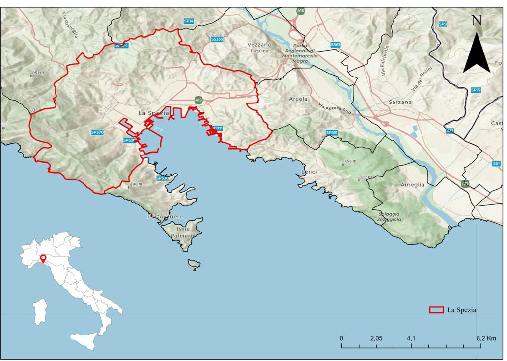
The dataset comprises 138 residential property sale deeds from the province of La Spezia, located in Northwestern Italy, covering transactions that occurred between 2004 and 2021 (see Figure 1). The properties are classified according to the Italian cadastral system as follows: A/1 (luxury dwellings situated in prestigious areas, characterized by high-end construction features and fine finishes), representing 1% of the sample; A/2 (standard residential units intended for civilian use), accounting for 73%; and A/3 (economically accessible housing), comprising the remaining 26%. Information on property prices and intrinsic attributes (as reported in Table 1) has been made available for analysis by the Italian Institute for Resources for Economic Development (IIRISE), a society operating in the field of properties valuation and managing a real estate database named “Comparabilitalia.it®” that stores information on properties that have been sold, allowing for market trend analysis and accurate real estate valuations1. Given that the sales occurred across different years, all property prices have been adjusted to May 2022 values using consumer price indices2.
| Variable | Unit of measurement | Source | Mean (or percentage) |
Standard deviation | Min | Max | |||||||||||||
|---|---|---|---|---|---|---|---|---|---|---|---|---|---|---|---|---|---|---|---|
| Price of sale (May 2022) | € | (a) | 220,987 | 157,866 | 194,648 | 247,326 | |||||||||||||
| Age of the property | Years | (a) | 54.17 | 34.95 | 7.00 | 350.00 | |||||||||||||
| Renovated property | (1 if yes) | (a) | 67.00% | ||||||||||||||||
| Cadastral class | (1 if A/3) | (a) | 26.00% | ||||||||||||||||
| Property surface | m2 | (a) | 96.60 | 43.71 | 24.30 | 299.00 | |||||||||||||
| Floor level | n. | (a) | 1.94 | 1.59 | 0.00 | 7.00 | |||||||||||||
| Property type_2 | (1 if bivans) | (a) | 5.00% | ||||||||||||||||
| Property type_3 | (1 if tree-rooms) | (a) | 17.00% | ||||||||||||||||
| Property type_4 | (1 if four-rooms) | (a) | 29.00% | ||||||||||||||||
| Property type_5 | (1 if six-rooms) | (a) | 25.00% | ||||||||||||||||
| Property type_6 | (1 if seven-rooms) | (a) | 16.00% | ||||||||||||||||
| Property type_7 | (1 if eight-rooms) | (a) | 8.00% | ||||||||||||||||
| judicial sale | (1 if yes) | (a) | 1.00% | ||||||||||||||||
| Energy category < B | (1 if yes) | (a) | 33.00% | ||||||||||||||||
| Years_restructuring services | years | (a) | 2021.78 | 0.41 | 2021.00 | 2022.00 | |||||||||||||
| Tavern | (1 if yes) | (a) | 1.00% | ||||||||||||||||
| Garage | (1 if yes) | (a) | 15.00% | ||||||||||||||||
| Uncovered parking space | (1 if yes) | (a) | 6.00% | ||||||||||||||||
| Covered parking space | (1 if yes) | (a) | 7.00% | ||||||||||||||||
| Hill_area | (1 if located in a hill area) | (b) | 3.00% | ||||||||||||||||
| Distance from primary schools | m | (b) | 1596.23 | 1528.13 | 65.50 | 8337.90 | |||||||||||||
| Distance from highway entrance | m | (b) | 3011.47 | 2010.13 | 326.40 | 8729.40 | |||||||||||||
| Distance from historic places | m | (b) | 630.63 | 421.97 | 5.40 | 2128.80 | |||||||||||||
| Distance from the railway station | m | (b) | 2294.98 | 2663.87 | 101.90 | 17281.80 | |||||||||||||
| Distance from parking area | m | (b) | 444.06 | 1,048.02 | 12.10 | 8,444.90 | |||||||||||||
| Number of parking places in a 1 km buffer | m | (b) | 2.65 | 2.46 | 0.00 | 8.00 | |||||||||||||
| Distance from the cycleway | m | (b) | 997.10 | 2232.92 | 1.40 | 15,547.40 | |||||||||||||
| Distance from landfills | m | (b) | 10,084.88 | 5,207.52 | 1,947.90 | 25,287.30 | |||||||||||||
| Number of buildings with asbestos within a 1 km buffer | n. | (b) | 0.09 | 0.34 | 0.00 | 2.00 | |||||||||||||
| Number of leisure associations within a 1 km buffer | n. | (b) | 0.43 | 0.73 | 0.00 | 2.00 | |||||||||||||
| Number of sport clubs within a 1 km buffer | n. | (b) | 0.62 | 0.65 | 0.00 | 2.00 | |||||||||||||
| Number of reception services within a 1 km buffer | n. | (b) | 17.32 | 15.63 | 0.00 | 48.00 | |||||||||||||
| Number of food services within a 1 km buffer | n. | (b) | 0.00 | 0.00 | 0.00 | 0.00 | |||||||||||||
| CORINE10* | 1 if yes | (b) | 41.00% | ||||||||||||||||
| Seismic zone_2 | (1 if yes) | (b) | 18.12% | ||||||||||||||||
| Seismic zone_3 | (1 if yes) | (b) | 17.39% | ||||||||||||||||
| Seismic zone_4 | (1 if yes) | (b) | 50.00% | ||||||||||||||||
| Note: (a) IIRISE-Comparabilitalia; (b) our GIS elaborations. *The property falls in the CORINE Land Cover class n. 10 (discontinuous urban fabric). | |||||||||||||||||||
Additional contextual and territorial information was obtained through GIS elaboration of data provided by the geoportal of the Liguria Region3 and by IGISMAP4. Table 1 reports descriptive statistics for variables used in the analysis.
The econometric analysis followed three main steps (see Figure 2). The first step involved the selection of the spatial weight matrix, a fundamental component in spatial econometric models that represents the spatial relationships among geographic units. This matrix defines, a priori, the structure of spatial dependence by assigning weights to pairs of observations based on their geographical proximity or connectivity. The choice of the weight matrix is critical, as it determines which observations are considered “neighbors” and therefore potentially exert mutual influence. Given the limited geographical scope of the analysis and the objective of capturing local interactions, we adopted a first-order Queen contiguity matrix (Kopczewska, 2021). We verified that, compared to an Inverse Euclidean Distance Matrix, the contiguity-based matrix captures a higher level of spatial variability, as indicated by the squared value of Moran’s I statistic (Kopczewska, 2021). Moran’s I, along with associated Z-values and p-values, was estimated using a computational approach based on 10,000 random permutations.
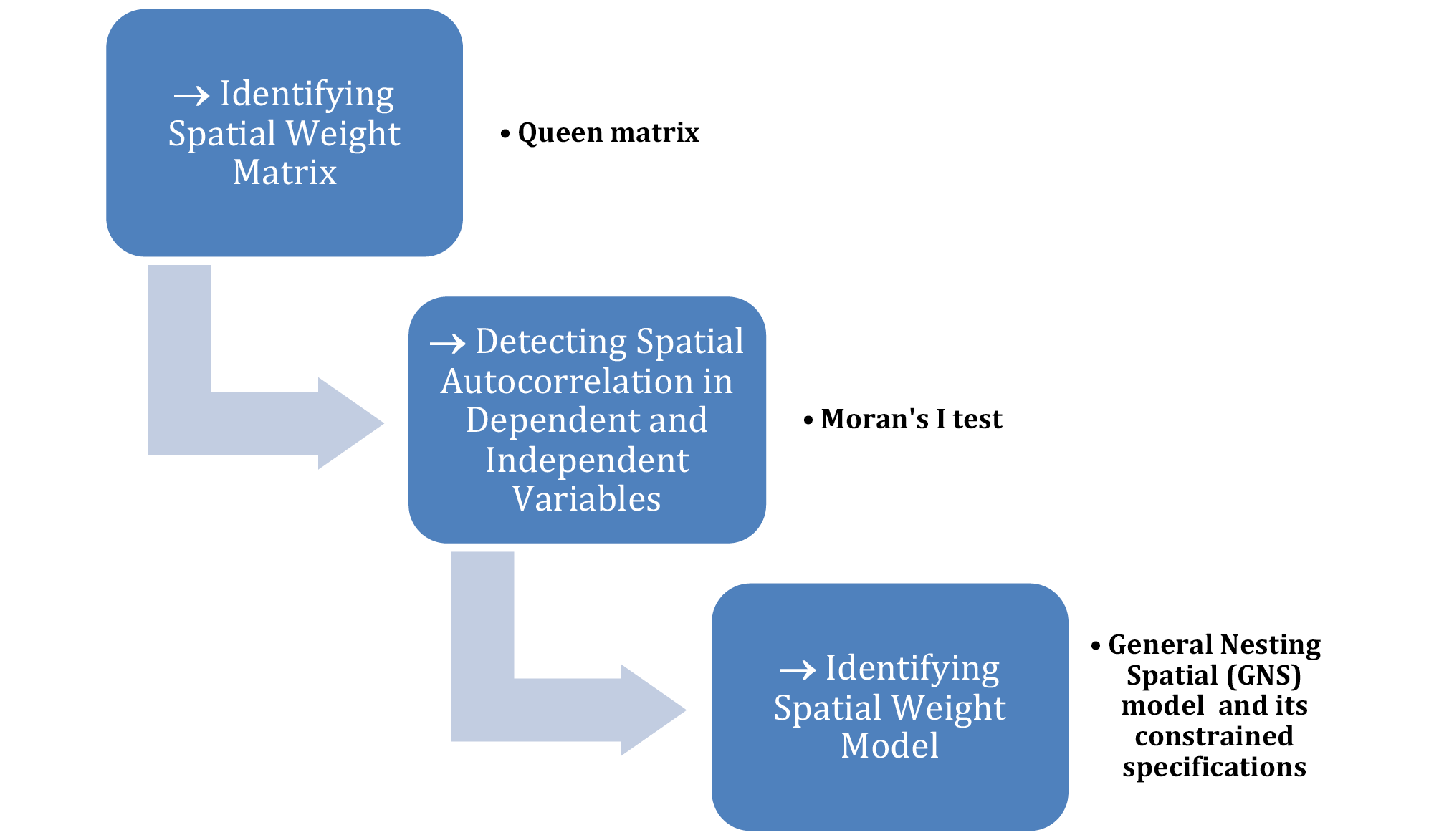
In the second step, we assessed the presence of spatial autocorrelation in both the dependent variable (property prices) and potential explanatory variables. Moran’s I statistic, Z-values, and p-values were computed using a Monte Carlo simulation approach based on 10,000 permutations. The detection of significant spatial dependence provided justification for the use of spatial econometric modelling. The selection of independent variables was guided by previous literature, particularly Algieri (2013).
In the final step, we followed the “general to specific” modelling strategy recommended by Elhorst (2010) to identify the most appropriate spatial model specification. This approach begins with the estimation of the General Nesting Spatial (GNS) model, originally proposed by Manski (1993). The GNS model incorporates three fundamental spatial lags: the spatial lag of the dependent variable (ρ), the spatial lag of independent variables (θ) and the spatial lag of the error term (λ). This comprehensive formulation allows for maximum flexibility in capturing various forms of spatial dependence. The general specification of the GNS model is as follows:
(1)
(2)
where:
–y is an Nx1 vector consisting of one observation on the dependent variable for every unit in the sample (i = 1, ..., 138);
–ρWyy represents the endogenous interaction effect where Wy is an N×N non-negative spatial weight matrix that defines the arrangement of the observational units in the sample, and ρ that is the spatial lag parameter capturing the strength of the spatial dependence in the dependent variable;
–iN is an N×1 vector of ones associated with the constant term parameter α;
–X denotes an N×K matrix of exogenous explanatory variables, with the associated parameters β contained in a K×1 vector;
–WxXθ represents the exogenous interaction effects, depending on Wx and on θ, that is the spatial Durbin parameter;
–λWuu represents the interaction effect among error terms, depending on Wu and on λ, that is the spatial error parameter;
–ε is the idiosyncratic error term.
As shown in Equation (1), a log-linear functional form was assumed to allow marginal effects to vary with the levels of the explanatory variables. This specification enables the interpretation of coefficients as elasticities, thereby capturing the non-linear relationship between property prices and their determinants.
The GNS model is a generalized model. Imposing restrictions on the value of spatial terms, it is possible to estimate other models that assume two or one spatial components. Generally, in the spatial econometric analysis, a satisfactory target is a model with two spatial factors, given that GNS often suffers from overspecification problems (Elhorst, 2014). Table 2 illustrates how reduced forms can be derived from the GNS by constraining the value of specific spatial term(s) to zero. These restricted models are the Spatial Autoregressive Combined (SAC) model, the Spatial Durbin Model (SDM), the Spatial Durbin Error Model (SDEM), the Spatial Autoregressive (SAR) model, the Spatial Lag of X (SLX) model, and the Spatial Error Model (SEM).
| Spatial Lag (ρ) |
Durbin Component (θ) |
Spatial Error (λ) |
|||||||||||||||||
|---|---|---|---|---|---|---|---|---|---|---|---|---|---|---|---|---|---|---|---|
| General Nesting Spatial (GNS) or Manski model | ≠ 0 | ≠ 0 | ≠ 0 | ||||||||||||||||
| Spatial Autoregressive Combined (SAC) or Keleijan-Prucha model | ≠ 0 | = 0 | ≠ 0 | ||||||||||||||||
| Spatial Durbin Model (SDM) | ≠ 0 | ≠ 0 | = 0 | ||||||||||||||||
| Spatial Durbin Error Model (SDEM) | = 0 | ≠ 0 | ≠ 0 | ||||||||||||||||
| Spatial Auto-Regressive (SAR) or spatial lag model | ≠ 0 | = 0 | = 0 | ||||||||||||||||
| Spatial Lag of X (SLX) model | = 0 | ≠ 0 | = 0 | ||||||||||||||||
| Spatial Error Model (SEM) | = 0 | = 0 | ≠ 0 | ||||||||||||||||
| Ordinary Least Squares (OLS) model | = 0 | = 0 | = 0 | ||||||||||||||||
| Source: adapted from Elhorst (2010). | |||||||||||||||||||
As suggested in literature (LeSage and Pace, 2014), models that include more than one spatial lag, must have the same spatial matrix for the three different spatial processes. That means that Wy = Wx = Wu = W, where W represents the best matrix specification selected as previously illustrated.
The spatial models were estimated using the Generalized Spatial Two-Stage Least-Squares (GS2LS) estimator, which provides consistent parameter estimates under both homoskedastic and heteroskedastic error structures (Drukker et al., 2013).
The analysis confirms that the adoption of the Queen contiguity matrix is appropriate for capturing spatial variability in property prices. Specifically, this matrix accounts for 9.08% of the variability in the dependent variable, compared to only 0.46% explained by the inverse Euclidean distance matrix. Using the Queen matrix, several contextual variables exhibit significant spatial autocorrelation. Table 3 presents the results of Moran’s I tests applied to these contextual variables, which, based on the relevant literature, are considered potential determinants of property sale prices.
| Moran’s I | z-value | ||
|---|---|---|---|
| Distance from primary schools | 0.5884 | 12.1145 | *** |
| Distance from the highway entrance | 0.8172 | 17.0035 | *** |
| Distance from historic places | 0.5655 | 12.2424 | **** |
| Distance from the railway station | 0.6936 | 14.7962 | *** |
| N. of leisure associations within a 1 km buffer | 0.8587 | 17.4973 | *** |
| N. of reception services within a 1 km buffer | 0.8472 | 17.7447 | *** |
| Distance from parking area | 0.6272 | 14.6769 | *** |
| N. of parking places in a 1 km buffer | 0.7107 | 14.5517 | *** |
| Distance from the cycleway | 0.6781 | 15.2375 | *** |
| N. of buildings with asbestos within a 1 km buffer | 0.607 | 13.6188 | *** |
| Seismic zone_2 | 0.4243 | 8.8786 | *** |
| Seismic zone_3 | 0.4967 | 10.0675 | *** |
| Seismic zone_4 | 0.7538 | 15.6493 | *** |
The findings indicate that the Spatial Durbin Error Model (SDEM) provides the best fit to the data, as it effectively accounts for spatial dependence in the error terms as well as exogenous interaction effects. Model comparison based on the Akaike Information Criterion (AIC) and the Bayesian Information Criterion (BIC) further supports the superiority of the SDEM specification. Table 4 reports the AIC and BIC values for all estimated models, clearly showing that the SDEM yields the most favorable performance metrics.
| Model | ll(model) | df | AIC | BIC | |||||||||||||||
|---|---|---|---|---|---|---|---|---|---|---|---|---|---|---|---|---|---|---|---|
| Maski | 4.97001 | 55 | 100.0600 | 261.0589 | |||||||||||||||
| SAC | -24.83119 | 42 | 133.6624 | 256.6070 | |||||||||||||||
| SDM | -6.138362 | 54 | 120.2767 | 278.3484 | |||||||||||||||
| SDEM | 4.721653 | 54 | 98.5567 | 256.6284 | |||||||||||||||
| SLX | -6.697225 | 52 | 117.3945 | 269.6116 | |||||||||||||||
| SEM | -25.69836 | 41 | 133.3967 | 253.4141 | |||||||||||||||
| SAR | -25.06558 | 40 | 130.1312 | 247.2213 | |||||||||||||||
| OLS | -25.76609 | 37 | 125.5322 | 233.8406 | |||||||||||||||
| * AIC and BIC Criteria were estimated using the Maximum Log-Likelihood estimator. | |||||||||||||||||||
Table 5 reports the coefficient estimates of the SDEM specification, as well as estimates of its direct and indirect effects. The estimates are consistent with the findings of previous aspatial studies, reinforcing the validity of the identified relationships between property prices and their determinants (Andreson and West, 2006; Ruggeri et al., 2023; Trojanek et al., 2018; Wong et al., 2011). Typical intrinsic characteristics – such as the age and size of the property, floor level, energy efficiency classification, and the presence of additional or ancillary spaces – emerge as key determinants of property prices. Furthermore, market segmentation based on property type and cadastral classification, as well as the conditions under which the transaction occurred (e.g., judicial sale), also significantly influence pricing dynamics (Simonotti, 2006).
| Coefficient estimates | Direct effect | Indirect effect | |||||||||||||||||
|---|---|---|---|---|---|---|---|---|---|---|---|---|---|---|---|---|---|---|---|
| β | Std. Err. | θ | Std. Err. | dy/dx | Std. err | dy/dx | Std. Err. | ||||||||||||
| Age of the property | -0.0022 | *** | 0.0006 | -0.0022 | *** | 0.0006 | |||||||||||||
| Renovated property | 0.1451 | ** | 0.0530 | 0.1451 | ** | 0.0530 | |||||||||||||
| Cadastral class | -0.3616 | *** | 0.0527 | -0.3616 | *** | 0.0527 | |||||||||||||
| Property surface | 0.0073 | *** | 0.0015 | 0.0073 | *** | 0.0015 | |||||||||||||
| Floor level | 0.0934 | *** | 0.0183 | 0.0934 | *** | 0.0183 | |||||||||||||
| Property type_2 | 0.7009 | ** | 0.2275 | 0.7009 | ** | 0.2275 | |||||||||||||
| Property type_3 | 0.9927 | *** | 0.2045 | 0.9927 | *** | 0.2045 | |||||||||||||
| Property type_4 | 1.0134 | *** | 0.2210 | 1.0134 | *** | 0.2210 | |||||||||||||
| Property type_5 | 1.0480 | *** | 0.2336 | 1.0480 | *** | 0.2336 | |||||||||||||
| Property type_6 | 1.1003 | *** | 0.2768 | 1.1003 | *** | 0.2768 | |||||||||||||
| Property type_7 | 1.0019 | *** | 0.2995 | 1.0019 | *** | 0.2995 | |||||||||||||
| Judicial sale | -0.6302 | ** | 0.2169 | -0.6302 | ** | 0.2169 | |||||||||||||
| Energy category | -0.1832 | ** | 0.0693 | -0.1832 | ** | 0.0693 | |||||||||||||
| Tavern | 0.3747 | ** | 0.1302 | 0.3747 | ** | 0.1302 | |||||||||||||
| Garage | 0.1577 | * | 0.0766 | 0.1577 | * | 0.0766 | |||||||||||||
| Uncovered parking space | 0.2224 | (a) | 0.1151 | 0.2224 | (a) | 0.1151 | |||||||||||||
| Covered parking space | 0.3215 | ** | 0.1213 | 0.3215 | ** | 0.1213 | |||||||||||||
| Hill_area | 0.8116 | * | 0.3491 | 0.8116 | * | 0.3491 | |||||||||||||
| Distance from historic places | -0.0004 | *** | 0.0001 | -0.0004 | *** | 0.0001 | |||||||||||||
| N. of reception services within a 1 km buffer | -0.0084 | ** | 0.0031 | -0.0084 | ** | 0.0031 | |||||||||||||
| N. of parking places in a 1 km buffer | 0.0453 | ** | 0.0173 | 0.0453 | ** | 0.0173 | |||||||||||||
| N. of buildings with asbestos within a 1 km buffer | -0.1895 | ** | 0.0615 | -0.1895 | ** | 0.0615 | |||||||||||||
| Distance from primary schools | -0.0001 | *** | 0.0000 | 0.0000 | *** | 0.0000 | -0.0001 | *** | 0.0000 | 0.0003 | *** | 0.0000 | |||||||
| N. of leisure associations within a 1 km buffer | -0.3071 | *** | 0.0804 | 0.0651 | *** | 0.0173 | -0.3071 | *** | 0.0804 | 0.4094 | *** | 0.1086 | |||||||
| Distance from highway entrance | 0.0002 | *** | 0.0000 | 0.0000 | *** | 0.0000 | 0.0002 | *** | 0.0000 | -0.0003 | *** | 0.0000 | |||||||
| Distance from the parking area | -0.0002 | *** | 0.0000 | 0.0001 | *** | 0.0000 | -0.0002 | *** | 0.0000 | 0.0008 | *** | 0.0001 | |||||||
| Distance from the cycleway | -0.0001 | *** | 0.0000 | 0.0000 | ** | 0.0000 | -0.0001 | *** | 0.0000 | -0.0002 | ** | 0.0001 | |||||||
| Seismic zone_2 | -0.2305 | ** | 0.0810 | 0.0983 | *** | 0.0204 | -0.2305 | ** | 0.0810 | 0.6180 | *** | 0.1285 | |||||||
| α | 10.5861 | *** | 0.3348 | ||||||||||||||||
| λ | -0.0958 | ** | 0.0355 | ||||||||||||||||
| Note: p<0.10, **p<0.05, *** p<0.001. | |||||||||||||||||||
Particularly noteworthy are the results related to contextual variables, as well as the sign and magnitude of the estimated direct and spillover effects – made possible when the spatial parameter associated with a given contextual variable is statistically significant. The effects of these variables are consistent with theoretical expectations and align with findings from previous studies in the literature (Crompton, 2001; Hidano et al., 2015; Rosiers et al., 2001; Seo et al., 2014).
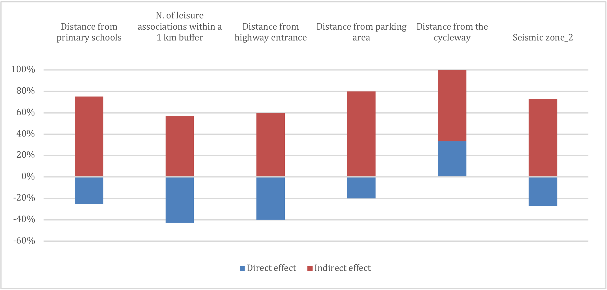
The spillover effect reinforces the direct effect only in the case of the variable “distance from the cycleway” which exhibits a negative total effect on property prices. In contrast, the remaining contextual variables generally exhibit spillover effects that are opposite in sign to their direct effects. For instance, variables such as the distance from primary schools, the number of leisure associations within a 1 km buffer, the distance from parking areas, and inclusion in seismic zone 2 (compared to other zones) display negative direct effects on property prices. However, these effects are partially offset by positive spillover effects from neighbouring areas. Conversely, the distance from the highway entrance shows a positive direct effect but is accompanied by a negative spillover effect. Moreover, as illustrated in Figure 3, for variables exhibiting a statistically significant Durbin component, the total effect is predominantly driven by the indirect component. These findings highlight the critical importance of accounting for both the direction and magnitude of spillover effects in order to fully understand the spatial dynamics governing property prices and their determinants.
6. Discussion and concluding remarks
The identification of property price determinants empowers stakeholders to make informed decisions, adapt to evolving real estate market conditions, and design effective management strategies that address the complex interplay of environmental, technological, social, and economic challenges affecting urban and settlement systems. Appraisers can also benefit from this information by producing valuation judgments that more accurately reflect the actual functioning of the real estate market, align with the expectations of buyers and sellers, and consider the spatial context in which the transaction may occur. By employing spatial econometric models and tools, researchers and practitioners can more effectively investigate which intrinsic and extrinsic factors significantly influence residential property prices. These models allow for the estimation of both the direction and magnitude of key relationships, while also accounting for spillover effects associated with spatially relevant variables. Spatial econometric models offer a nuanced understanding of the factors influencing property values, capturing not only the direct effects of explanatory variables but also the spatial interactions among neighbouring units. This methodological approach is consistent with a growing body of literature that underscores the role of sustainability measures – such as energy efficiency and decarbonization – in enhancing property values. Additionally, recent studies highlight the importance of specific property uses in promoting urban regeneration and generating positive externalities that extend beyond individual property boundaries. In the context of real estate market analysis and property appraisal, spatial econometric tools demonstrate the critical importance of accounting for spatial autocorrelation in the data. These models enhance the accuracy, reliability, and policy relevance of economic analyses by reducing the risk of coefficient bias – whether through underestimation or overestimation – and by improving the predictive validity of market value estimates. Ultimately, spatial econometric methods provide valuable support in explaining how and why property prices vary across space, and in identifying the underlying processes driving these spatial patterns. This paper presents the results of a spatial econometric hedonic analysis aimed at identifying the factors influencing residential property prices in La Spezia, Italy. The findings indicate that the Spatial Durbin Error Model (SDEM) provides the best-fitting specification, supporting the hypothesis of significant spatial dependence both in the error terms and in the interaction effects of exogenous variables. The results of this study emphasize the critical need for urban planners and real estate professionals to account for both direct and spillover effects when evaluating property prices. Intrinsic characteristics like the asset’s age, size, and energy efficiency categories are key determinants and should be included as core variables in valuation models. Additionally, incorporating context variables (e.g., proximity to schools, highways, or cycleways) with spatial parameters allows for more accurate estimations that reflect spatial dependencies and interactions, aspects that cannot be ignored in real estate valuations. The significant spillover effects observed for certain variables – such as distance from the cycleway – suggest that investments in urban infrastructure can generate broader impacts beyond the immediate vicinity, influencing property values in surrounding areas. Urban planners can leverage this insight to prioritize infrastructure projects that are likely to yield positive spatial externalities. Conversely, the presence of negative spillover effects associated with factors such as distance from parking areas or location within seismic zones underscores the importance of implementing mitigation strategies, including improved accessibility and enhanced safety measures. Positive effects linked to proximity to leisure associations and cycleways further highlight the value of fostering community-oriented, sustainable urban environments. Such amenities not only enhance the attractiveness of neighbourhoods but also contribute to increased property values. In contrast, areas adversely affected by proximity to undesirable features – such as seismic risk zones – may benefit from compensatory policy measures, including development incentives or robust disaster resilience planning, to offset negative market perceptions. The findings also emphasize the importance of market segmentation – particularly with respect to property type and cadastral classification – in shaping price dynamics. This information can support policymakers and real estate developers in designing targeted interventions that address the specific characteristics and needs of distinct market subsegments.
The observed influence of judicial sales on property prices underscores the critical importance of accounting for legal and procedural factors in real estate transactions. These considerations should be consistent with the market value definition established by the European Union in Regulation (EU) No 575/2013. Accordingly, this analysis aligns with findings from similar studies and emphasizes that failure to adhere to valuation standards – particularly in the selection of comparable properties – can result in significant distortions in price estimations. To operationalize these findings, it is essential that local governments and analysts have access to high-quality spatial data. Such data should encompass both intrinsic property characteristics and contextual variables with sufficient granularity to enable the accurate estimation of spatial interactions. Geographic Information Systems (GIS) can support this effort by facilitating the visualization and analysis of spatial relationships, thereby helping stakeholders to identify priority areas for targeted interventions. Incorporating both direct and spillover effects into urban planning and real estate valuation processes can contribute to the development of more sustainable, resilient, and equitable urban environments.
The study is not without limitations. Its focus on residential properties within the province of La Spezia may limit the generalizability of the findings to other property types or different urban contexts. Additionally, the analysis does not account for broader macroeconomic influences or regional policy interventions that may affect real estate dynamics. Nevertheless, despite these limitations, the study provides a robust foundation for analysing local housing markets and offers valuable insights to inform future research and policy development. Future research could build on this analysis by integrating additional explanatory variables and incorporating more recent and comprehensive datasets. Expanding the geographical scope to include other medium-sized cities or different property types – such as commercial and industrial real estate – would facilitate a broader understanding of spatial dynamics across diverse urban contexts. Moreover, extending the temporal dimension of the dataset or incorporating more frequent updates would enable the examination of long-term trends, the impact of economic cycles, and the effects of external shocks on property markets. Further contributions could include an investigation into the spatial effects of urban regeneration initiatives and the repurposing of underutilized or vacant properties, which remain underexplored in the literature. Integrating social, demographic, and environmental indicators would also provide a more comprehensive understanding of the multifaceted drivers of property values. Finally, future studies could benefit from employing advanced spatial econometric techniques capable of capturing more complex relationships and interactions within the data.
Aladwan, Z., & Ahamad Mohd, S. S. (2019). The hedonic pricing model for real property valuation via GIS-A review. Civil and Environmental Engineering Reports, 29(3), 34–47.
Algieri, B. (2013). House price determinants: fundamentals and underlying factors. Comparative Economic Studies, 55, 315–341.
American Institute of Real Estate Appraisers. (1952). The Appraisal of Real Estate. The Institute.
Anderson, S. T., & West, S. E. (2006). Open space, residential property values, and spatial context. Regional Science and Urban Economics, 36(6), 773–789.
Anselin, L. (2022). Spatial econometrics. In Rey, S. J., & Franklin, R. (Eds.). Handbook of spatial analysis in the social sciences, pp. 101-122. Cheltenham, Edward Elgar Publishing.
Arcuri, N., De Ruggiero, M., Salvo, F., & Zinno, R. (2020). Automated valuation methods through the cost approach in a BIM and GIS integration framework for smart city appraisals. Sustainability, 12(18), 7546.
Aziz, A., Anwar, M. M., Abdo, H. G., Almohamad, H., Al Dughairi, A. A., & Al-Mutiry, M. (2023). Proximity to neighborhood services and property values in urban area: An evaluation through the hedonic pricing model. Land, 12(4), 859.
Barreca, A., Curto, R., & Rolando, D. (2018). Housing vulnerability and property prices: spatial analyses in the Turin real estate market. Sustainability, 10(9), 3068.
Belke, A., & Keil, J. (2018). Fundamental determinants of real estate prices: a panel study of German regions. International Advances in Economic Research, 24, 25–45.
Bernknopf, R., Gillen, K., Wachter, S., & Wein, A. (2010). Using econometrics and geographic information systems for property valuation: a spatial hedonic pricing model. In Linne, M., & Thompson, M. (Eds.). Visual valuation: implementing valuation modeling and geographic information solutions. Chicago, Appraisal Institute, 265–300.
Bocci, C., Ferretti, C., & Lattarulo, P. (2019). Spatial interactions in property tax policies among Italian municipalities. Papers in Regional Science, 98(1), 371–392.
Bolitzer, B., & Netusil, N. R. (2000). The impact of open spaces on property values in Portland, Oregon. Journal of Environmental Management, 59(3), 185–193.
Caliman, T., & Di Bella, E. (2011). Spatial autoregressive models for house price dynamics in Italy. Economics Bulletin, 31(2), 1837–1855.
Can, A. (1990). The measurement of neighborhood dynamics in urban house prices. Economic Geography, 66(3), 254–272.
Case, B., Clapp, J., Dubin, R., & Rodriguez, M. (2004). Modeling spatial and temporal house price patterns: a comparison of four models. The Journal of Real Estate Finance and Economics, 29, 167–191.
Chang, L. C., & Lin, H. Y. (2012). The impact of neighborhood characteristics on housing prices-an application of hierarchical linear modeling. International Journal of Management and Sustainability, 1(2), 31.
Chau, K. W., & Chin, T. L. (2003). A critical review of literature on the hedonic price model. International Journal for Housing Science and its applications, 27(2), 145–165.
Chen, Y., Jones, C. A., Dunse, N. A., Li, E., & Liu, Y. (2023). Housing prices and the characteristics of nearby green space: Does landscape pattern index matter? evidence from metropolitan area. Land, 12(2), 496.
Cipollini, A., & Parla, F. (2020). Housing market shocks in Italy: a GVAR approach. Journal of Housing Economics, 50, 101707.
Copiello, S. (2020). Spatial dependence of housing values in Northeastern Italy. Cities, 96, 102444.
Crompton, J. L. (2001). The impact of parks on property values: a review of the empirical evidence. Journal of Leisure Research, 33(1), 1–31.
Cunha, A. M., & Lobão, J. (2021). The determinants of real estate prices in a European context: a four-level analysis. Journal of European Real Estate Research, 14(3), 331–348.
De Noni, I., Ghidoni, A., Menzel, F., Bahrs, E., & Corsi, S. (2019). Exploring drivers of farmland value and growth in Italy and Germany at regional level. Aestimum, 74, 77–99.
De Ruggiero, M., & Salvo, F. (2011). Misure di similarità negli adjustment grid methods. Aestimum, 58, 47–58.
De Toro, P., Nocca, F., Renna, A., & Sepe, L. (2020). Real estate market dynamics in the city of Naples: an integration of a multi-criteria decision analysis and geographical information system. Sustainability, 12(3), 1211.
Drukker, D. M., Prucha, I. R., & Raciborski, R. (2013). Maximum likelihood and generalized spatial two-stage least-squares estimators for a spatial-autoregressive model with spatial-autoregressive disturbances. The Stata Journal, 13(2), 221–241.
Durst, N. J., Sullivan, E., & Jochem, W. C. (2024). The spatial and social correlates of neighborhood morphology: Evidence from building footprints in five US metropolitan areas. Plos one, 19(4), e0299713.
Elhorst, J. P. (2010). Applied spatial econometrics: raising the bar. Spatial Economic Analysis, 5(1), 9–28.
Elhorst, J. P. (2014). Spatial econometrics: from cross-sectional data to spatial panels. Heidelberg, Springer.
European Construction Sector Observatory (2019). Housing affordability and sustainability in the EU. Analytical report. Available at: https://single-market-economy.ec.europa.eu/sectors/construction/observatory/analytical-reports_en (Accessed 10 September 2024).
Fingleton, B. (2006). A cross‐sectional analysis of residential property prices: the effects of income, commuting, schooling, the housing stock and spatial interaction in the English regions. Papers in Regional Science, 85(3), 339–361.
Ganduri, R., Xiao, S. C., & Xiao, S. W. (2023). Tracing the source of liquidity for distressed housing markets. Real Estate Economics, 51(2), 408–440.
Giuffrida, L., De Salvo, M., Manarin, A., Vettoretto, D., & Tempesta, T. (2023). Exploring farmland price determinants in Northern Italy using a spatial regression analysis. Aestimum, 83, 3–20.
Guan, C., & Peiser, R. B. (2018). Accessibility, urban form, and property value. Journal of Transport and Land Use, 11(1), 1057–1080.
Herath, S., & Maier, G. (2010). The hedonic price method in real estate and housing market research: a review of the literature. WU Vienna University of Economics and Business. SRE - Discussion Papers No. 2010/03
Hidano, N., Hoshino, T., & Sugiura, A. (2015). The effect of seismic hazard risk information on property prices: evidence from a spatial regression discontinuity design. Regional Science and Urban Economics, 53, 113–122.
Jin, S., Zheng, H., Marantz, N., & Roy, A. (2024). Understanding the effects of socioeconomic factors on housing price appreciation using explainable AI. Applied Geography, 169, 103339.
Kishor, N. K. (2022). Comovements and spillovers in international commercial and residential real estate markets. Journal of European Real Estate Research, 15(3), 311–331.
Lee, C. C., Liang, C. M., Yeh, W. C., & Yu, Z. (2022). The impact of urban renewal on neighboring housing prices: An application of hierarchical linear modeling. International Journal of Strategic Property Management, 26(1), 1123.
LeSage, J. P., & Pace, R. K. (2014). The biggest myth in spatial econometrics. Econometrics, 2(4), 217–249.
Li, J., Zheng, L., Liu, C., & Shen, Z. (2021). Information spillover effects of real estate markets: evidence from ten metropolitan cities in China. Journal of Risk and Financial Management, 14(6), 244.
Lindsey, G., Payton, S., Man, J., & Ottensmann, J. (2003). Public choices and property values: evidence from Greenways in Indianapolis. Indianapolis: Center for Urban Policy and the Environment. 12 p.
Lo, D., Chau, K. W., Wong, S. K., McCord, M., & Haran, M. (2022). Factors affecting spatial autocorrelation in residential property prices. Land, 11(6), 931.
Locurcio, M., Morano, P., Tajani, F., & Di Liddo, F. (2020). An innovative GIS-based territorial information tool for the evaluation of corporate properties: An application to the Italian context. Sustainability, 12(14), 5836.
Mahan, B. L., Polasky, S., & Adams, R. M. (2000). Valuing urban wetlands: a property price approach. Land Economics, 76(1), 100–113.
Manski, C. F. (1993). Identification of endogenous social effects: the reflection problem. The Review of Economic Studies, 60(3), 531–542.
Marinković, S., Džunić, M., & Marjanović, I. (2024). Determinants of housing prices: Serbian Cities’ perspective. Journal of Housing and the Built Environment, 39(3), 1601–1626.
Morena, M., Cia, G., Baiardi, L., & Rodríguez Rojas, J. S. (2021). Residential property behavior forecasting in the metropolitan city of Milan: socio-economic characteristics as drivers of residential market value trends. Sustainability, 13(7), 3612.
Musa, U. S. M. A. N., & Yusoff, W. Z. W. (2015). Impact of neighborhood characteristics on residential property values: a critical review of literature. International Review of Social Sciences, 3(4), 147–155.
Musa, U., & Yusoff, W. Z. W. (2017). The influence of housing components on prices of residential houses: a review of literature. The Social Sciences, 12(4), 625–632.
Osland, L., Östh, J., & Nordvik, V. (2022). House price valuation of environmental amenities: an application of GIS‐derived data. Regional Science Policy & Practice, 14(4), 939–959.
Paraschiv, C., & Chenavaz, R. (2011). Sellers’ and buyers’ reference point dynamics in the housing market. Housing Studies, 26(03), 329–352.
Poulhes, M. (2018). From Latin Quarter to Montmartre: Investigating Parisian Real Estate Prices. Annals of Economics and Statistics/Annales d’Économie et de Statistique, 130, 39–68.
Riccioli, F., Fratini, R., & Boncinelli, F. (2021). The impacts in real estate of landscape values: evidence from Tuscany (Italy). Sustainability, 13(4), 2236.
Rosato, P., Breil, M., Giupponi, C., & Berto, R. (2017). Assessing the impact of urban improvement on housing values: a hedonic pricing and multi-attribute analysis model for the historic centre of Venice. Buildings, 7(4), 112.
Rosiers, F. D., Lagana, A., & Theriault, M. (2001). Size and proximity effects of primary schools on surrounding house values. Journal of Property Research, 18(2), 149–168.
Ruggeri, A. G., Gabrielli, L., Scarpa, M., & Marella, G. (2023). What is the impact of the energy class on market value assessments of residential buildings? An analysis throughout Northern Italy based on extensive data mining and artificial intelligence. Buildings, 13(12), 2994.
Salvo, F., De Ruggiero, M., & Tavano, D. (2022). Social variables and real estate values: the case study of the City of Cosenza. In Napoli, G., Mondini, G., Oppio, A., Rosato, P., & Barbaro, S. (Eds.). Values, Cities and Migrations: Real Estate Market and Social System in a Multi-cultural City. pp. 173-186. Cham, Springer International Publishing.
Salvo, F., Tavano, D., & De Ruggiero, M. (2021). Hedonic price of the built-up area appraisal in the market comparison approach. In Bevilacqua, C., Calabrò, F., & Della Spina, L. (Eds.). New Metropolitan Perspectives: Knowledge Dynamics and Innovation-driven Policies Towards Urban and Regional Transition Volume 2. pp. 696-704. Cham, Springer International Publishing.
Sani, A., Mohammed, M. I., & Usman, H. (2023). Locational, neighbourhood and physical characteristics of residential rental properties: a review. Journal of Commerce, Management, and Tourism Studies, 2(3), 143–154.
Seo, K., Golub, A., & Kuby, M. (2014). Combined impacts of highways and light rail transit on residential property values: a spatial hedonic price model for Phoenix, Arizona. Journal of Transport Geography, 41, 53-62.
Seo, Y. (2020). Varying effects of urban tree canopies on residential property values across neighborhoods. Sustainability, 12(10), 4331.
Sica, F., Tajani, F., & Cerullo, G. (2025). An evaluation model for an optimal decarbonisation process in the built environment. Built Environment Project and Asset Management, 15(1), 51–66.
Simonotti, M. (2006). Metodi di stima immobiliare. Applicazione degli standard internazionali. Palermo, Dario Flaccovio.
Stamou, M., Mimis, A., & Rovolis, A. (2017). House price determinants in Athens: a spatial econometric approach. Journal of Property Research, 34(4), 269–284.
Tajani, F., Manganelli, B., Cerullo, G., Morano, P., & Morente, M. A. (2023, June). The student housing as a catalyst for virtuous processes of “win-win” revitalization of property assets in disuse. In Gervasi, O., Murgante, B., Rocha, A. M. A. C., Garau, C., Scorza, F., Karaca, Y., Torre, C. M. (Eds.). Computational Science and Its Applications – ICCSA 2023 Workshops. ICCSA 2023. Lecture Notes in Computer Science, vol 14109. pp. 387-400. Cham, Springer.
Trojanek, R., Gluszak, M., & Tanas, J. (2018). The effect of urban green spaces on house prices in Warsaw. International Journal of Strategic Property Management, 22(5), 358–371.
Vergos, K. P., & Zhi, H. (2018). Is it a curse or a blessing to live near rich neighbors? Spatial analysis and spillover effects of house prices in Beijing. Spatial Analysis and Spillover Effects of House Prices in Beijing (November 22, 2018).
Wang, Y., Wang, S., Li, G., Zhang, H., Jin, L., Su, Y., & Wu, K. (2017). Identifying the determinants of housing prices in China using spatial regression and the geographical detector technique. Applied Geography, 79, 26–36.
Wong, S. K., Chau, K. W., Yau, Y., & Cheung, A. K. C. (2011). Property price gradients: the vertical dimension. Journal of Housing and the Built Environment, 26, 33–45.
Zhang, Y., Zhang, D., & Miller, E. J. (2021). Spatial autoregressive analysis and modeling of housing prices in city of Toronto. Journal of Urban Planning and Development, 147(1), 05021003.
Zihannudin, N. Z., Maimun, N. H. A., & Ibrahim, N. L. (2021). Brownfield sites and property market sensitivity. Planning Malaysia, 19(2), 121–130.
Zoppi, C., Argiolas, M., & Lai, S. (2015). Factors influencing the value of houses: estimates for the city of Cagliari, Italy. Land Use Policy, 42, 367–380.
1 The Comparabilitalia database contains data derived from approximately 1,500,000 geolocated property sale deeds, which are integrated with cadastral information. These data are primarily utilized by professionals involved in appraisal activities, who access the information through a user-friendly, subscription-based platform (https://comparabilitalia.it).