Classification of products based on the uncertainty of supply chain demand: a case study of wineries in Chile
1 Universidad de Lleida; Plaça de Víctor Siurana, 1, 25003 Lleida, España
2 Universidad Santiago de Chile, Avenida Libertador Bernardo O’Higgins 3363, Estación Central, Santiago 9160000, Chile
*Corresponding author. Email: scmchile@gmail.com
Abstract. The wine industry faces distinctive supply chain challenges, including high product variety, export market fragmentation, and seasonal production, all of which contribute to demand uncertainty. Importantly, this uncertainty is not only externally driven but also amplified by tactical and operational decisions – such as labeling, bottling strategies, and product customization – that increase complexity. This study presents a product classification methodology based on demand behavior to improve decision-making in inventory management. Using a case study of three Chilean wineries located in the Central Valley, we compare the traditional ABC classification – commonly used in ERP systems – with a quantitative model that incorporates demand variability. The proposed approach enables segmenting products according to average demand and variability, offering clearer insights for setting differentiated service levels, inventory policies, and forecasting strategies. The findings show that the demand uncertainty-based classification provides more effective support for supply chain decision-making than conventional methods. The model has also demonstrated applicability beyond finished goods, such as in-process wine and critical inputs like corks and bottles. This research contributes empirical evidence to close the gap between theory and practice, providing a replicable tool for product segmentation in wine and other industries facing demand complexity.
Keywords: demand uncertainty, wine supply chain, production and inventory management, product classification, wine industry.
Index
3.2 Selection of quantitative methods
4.1 Quantitative classification
4.2 Finished product variability Winery V1
4.3 Variability of the finished products of Winery V2
4.4 Variability of the finished products of Winery V3
4.5 Variability of finished products ABC of Winery V1
The wine industry faces distinctive supply chain challenges that are shaped by factors such as seasonal production, market volatility, export dependency, and regulatory frameworks. These dynamics make inventory planning and demand forecasting particularly complex, especially in export-oriented wine-producing countries like Chile. According to [1], vineyards in Chile’s Central Valley exhibit diverse economic performance linked to their operational management and exposure to international markets. Moreover, [2] show that climate variability adds a further layer of uncertainty to the sector, influencing both production volume and quality.
Despite growing research on supply chain resilience in the wine industry [3], few studies have addressed how demand-side uncertainty impacts inventory classification and decision-making. Most prior work has focused on managing supply-related uncertainty or improving vineyard operations. For instance, [3] explore strategic responses to supply disruptions, while [4] examine the adoption of Lean Six Sigma in Italian wineries to enhance supply chain performance under regulatory and environmental pressure.
Previous studies have raised the need for further research into new approaches to uncertainty modeling, to obtain new approaches to production planning and control to manage uncertainty within each supply chain company, the incorporation of all types of uncertainty in an integrated manner, and the development of empirical work comparing different modeling approaches with real case studies [5]. In addition, [6] emphasizes the need to conduct empirical research on the uncertainties that occur in a particular industrial context and the most effective management actions in reducing one or more of the key uncertainties.
Uncertainty impacts production practices and supply chain performance [7]. Given the potential problems, interest in supply chain decisions that take uncertainty and risk into account has increased [8,9].
However, the application of quantitative classification techniques that explicitly incorporate demand variability - particularly in the context of inventory management - remains limited in wine economics literature. Traditional ABC classification is widely used in Enterprise Resource Planning (ERP) systems, yet it fails to account for volatility in demand patterns. This omission can hinder the efficiency of inventory allocation in wineries that handle a diverse portfolio of products across domestic and export markets.
This paper addresses this gap by proposing a classification approach based on demand uncertainty and comparing it with the traditional ABC method. Using a case study of three Chilean wineries, we assess the effectiveness of a variability-driven model for categorizing products and guiding inventory decisions. Our findings aim to inform winery managers and supply chain practitioners of new tools that support operational efficiency in the face of fluctuating demand. By contextualizing the research within the wine industry and referencing sector-specific studies, we contribute to bridging the theoretical and practical knowledge on inventory management under uncertainty.
Product classification should be part of a comprehensive inventory management system. Figure 1 shows an adaptation of the 4-stage model proposed by [10]. This research focuses on the first stage of product classification.

Our work focuses on showing the contrast of empirical use with theoretical techniques and we seek to contribute to closing the gap between theoretical research on supply chain uncertainty management and practice.
In this literature review we go through quantitative methods for classifying products in order to tailor supply chain operational decisions.
A supply chain is composed of all parties involved, directly or indirectly, to satisfy a customer’s order. The supply chain includes not only the manufacturer and suppliers, but also transporters, distributors, retailers, and even the customers themselves, as shown in Figure 2. A supply chain is dynamic and involves the constant flow of information, products, and money between different stages. The primary purpose of any supply chain is to satisfy customer needs, and in the process, generate a profit for itself. The success of a supply chain should be measured in terms of its profitability rather than profit at an individual stage [11–13].

All processes in a supply chain fit into two categories in relation to end-customer demand: push or pull. Pull processes produce make to order, while push processes initiate execution in anticipation of customer orders based on a forecast and produce make to stock [14,15]
Global supply chain optimization is difficult because it needs to be designed and operated in which several factors contribute to uncertainty, including: 1. Matching supply and demand is a major challenge because production levels need to be committed well before demand is realized. 2. Inventory levels and order backlogs fluctuate considerably throughout the supply chain. 3. Forecasting does not solve the problem. 4. Demand is not the only source of uncertainty; lead times, manufacturing yields, transportation times, and component availability are also sources of uncertainty [16,17].
Supply chain uncertainty refers to decision making in which the decision maker does not know definitively what to decide because he/she is confused about the objectives; lacks information about the supply chain or its environment; lacks information processing capabilities; cannot accurately predict the impact of possible control actions; or lacks effective control actions [18].
It has been suggested that demand uncertainty and implied demand uncertainty represent distinct concepts [11]. Demand uncertainty reflects the uncertainty of customer demand for a product. Implicit demand uncertainty is that resulting from the way the customer orders: if you serve only urgent orders, you will have a higher implicit uncertainty than if you deliver with long lead times. Uncertainty generates complexity in the supply chain, tends to increase inventory and propagates through the supply network [19,20]. Demand uncertainty is particularly important and tends to reduce profits in the supply chain [21].
It is expected that supply chain planning methods that do not include uncertainty will underperform those that do [22]. Both linear and circular supply chains must take uncertainty into account in their management [23].
Recent contributions in the wine industry have highlighted the importance of integrating sector-specific dynamics into supply chain analysis. The value of process improvement methodologies such as Lean Six Sigma in Italian wineries has been demonstrated [4], while preparedness for disruptions – a growing concern under increased climate volatility – has been addressed by [3] and [2]. Additionally, the influence of vineyard management strategies and environmental variability on performance in Chilean wine production has been explored in greater depth [1]. However, most of these studies have emphasized supply-side uncertainties and strategic resilience rather than the operational challenges linked to demand volatility.
Supply chain uncertainty management models are classified into 3: strategic, tactical, and operation [24,25]. The strategy time horizon is several years and decides the configuration of the supply chain, how resources will be allocated, and what processes each stage will perform [26,27]. The planning or tactical horizon is from one quarter to one year and includes demand forecasts, deciding which markets will be supplied from which locations, manufacturing outsourcing, inventory policies, timing, promotions and pricing. Planning also includes decisions regarding demand uncertainty, exchange rate, and competition [28,29]. The time horizon of the operation is daily or weekly, in this phase decisions are made regarding customer orders, allocating inventories or production to orders, setting order delivery dates, defining pick lists for a warehouse, assigning orders to shipments, establishing delivery schedules, etc. [30,31].
Supply chain demand uncertainty models can also be classified into qualitative and quantitative models according to the solution methodology [32]. And they can be classified by source of uncertainty: demand, supply and production processes [22,33].
Supply chain planning models under uncertainty have been studied [23], but they are not commonly related to product classification [22]. Inventory production planning and control systems classify products into those with independent or dependent demand. Finished products have independent demand, that which comes from customers and needs to be forecast. Raw materials and in-process products have dependent demand, and the demand is calculated based on the production of finished products [34,35].
The need to link product classification with inventory management systems in an integrated way has been raised in the literature [10,36].
A literature review of product classification based on various factors is presented in [37]. In particular, classifications can rely on either judgment-based (qualitative) or statistical (quantitative) techniques. The quantitative approaches include ABC classification and two-dimensional graphical matrices (2×2).
Among the quantitative classifications, the ABC classification is the most widespread as it is part of integrated ERP systems. This classification is based on the Pareto Principle, also known as the 80/20 rule, and was originally used to classify goods according to their annual demand. To calculate it, the annual demand is calculated and multiplied by the cost. Class A goods have 80% of the annual volume in money and account for 20% of the goods; Class B goods account for 15% of the annual volume in money and account for 30% of the goods; Class C accounts for 5% of the annual volume in money and comprises about 50% of the goods [38,39]. Multiple factors are considered for using ABC as annual usage value, e.g., average consumption, annual failures, and lead time [40].
The use of two-dimensional graphical matrices (2×2) in product classification is discussed in [37], referencing their application to spare parts [41,42] and to manufactured products [43]. Additionally, a similar matrix-based approach has been identified in the work of another author [44].
A 2×2 matrix-based quantitative classification method grounded in demand uncertainty was applied to a Chilean winery case in [45], demonstrating its superiority over traditional qualitative approaches such as those proposed by [46] and [47]. This study validates the usefulness of variability-based product classification models for supporting different production stages within a winery.
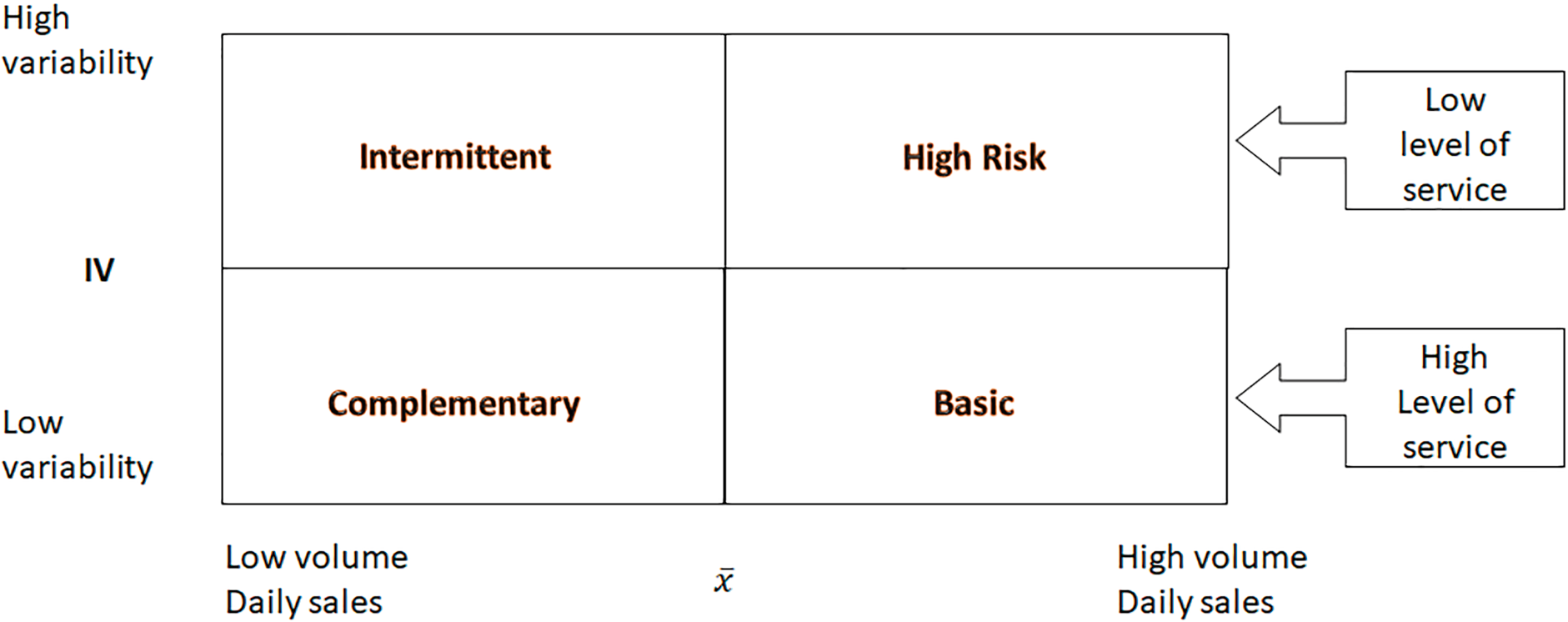
This quantitative method by [43,44] uses a two-dimensional matrix and allows measuring demand uncertainty. The two dimensions are the average daily sale in units and the variability index:
is the average daily sales in logarithmic scale
IV (variability index) = σ / is the standard deviation of the article in demand divided by the average sale.
Four product categories are identified:
– Basic: products with high volume demand and low variability. These are stable, predictable items, and in the case of finished products, they provide the greatest amount of income to the company.
– Complementary: products with low demand volume and low variability. They are also stable items and, in the case of finished products, provide low revenues on a regular basis.
– High risk: products with high volume demand and high variability.
– Intermittent: products with low demand volume but high variability.
The variability index is also known in the literature as coefficient of variability (CV) or (CoV) as an indicator to measure demand uncertainty [48,49].
In this research we use the case study method. [50] has posited that the case method is one of the most powerful methods in operations management research and has contributed from the development of lean manufacturing theory to manufacturing strategy.
We use the structure proposed by [50] to describe the methodology:
1. When to use case study research: the purpose of this research is to contribute to the testing of theory.
2. The research framework: In an inventory management system we focus on the product classification stage. We seek to identify whether the quantitative method of [43,44] which is based on demand uncertainty is better than other quantitative models such as ABC.
3. Choice of case: The case studies three wineries in Chile. The type of case would be retrospective.
4. Development of research instruments and protocols: Semi-structured interviews, meetings, visits to bottling facilities and wineries, and document analysis were designed for data collection. Also conduct data analysis of product sales transactions to obtain information for the quantitative model. The performance of the methods would be determined by user acceptance.
5. Conducting field research: The primary contact was the operations manager. The main informants were the head of planning, the production planners, and the operations manager.
6. Documentation and data coding: The first step was to identify the methods used by the company. In section 3.2 quantitative method selection, we explained how the quantitative methods were selected and applied to test their performance. We worked on Excel sheets.
7. Analysis. The analysis and its results were validated by the head of planning and the operations manager. In section 5. Discussion we compare the results of the 3 vineyards.
The three wineries selected for this study are located in Chile’s Central Valley, which is recognized as the country’s most important wine-producing region, both in terms of volume and international projection. This area concentrates a significant share of vineyard surface and export-oriented production, making it a strategic reference for understanding the operational and commercial dynamics of the Chilean wine industry [1]. The selected wineries represent diverse business models within this region – ranging from mid-sized exporters to producers with differentiated product portfolios – allowing us to examine how demand uncertainty affects inventory classification across different contexts within a shared geographical and market environment. We will call them wineries V1, V2 and V3 in order of SKU number.
The supply chain of a winery includes different stages: an agricultural stage for grape production, an oenology stage to produce wine from different grape varieties, a production stage for bottling the wine, domestic distribution or export, retail sales and the customer.
The vineyards own part of the grape production, winemaking, bottling production and finished product cellars; they do not own foreign distribution centers or retail sales.
The winemaking follows the production strategy make-to-stock because the wine needs to rest in barrels and because there are relatively few vines. Bottling follows a make-to-stock method for domestic sales and make-to-order for exports. For exports it is not possible to produce make-to-stock because international sales are very fragmented, and the product label is not standardized for the countries due to legal regulations related to the alcohol content allowed by the countries. The bottling and winemaking plants are located near the grape fields south of Santiago. Export shipments are made through the ports of Valparaíso and San Antonio about 115 km west of Santiago.
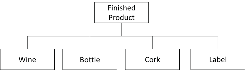
In this case we focus on the production of bottling for export. Supply chain management is concerned with determining the supply and production levels and inventories of raw materials, subassemblies at the different levels of the given bill of materials (BOM) [51]. The finished products use wine, bottle, cork, and label as the main raw materials as shown in Figure 4. All inputs except the label are kept in stock. The label must be printed when the customer’s order arrives. Since there are different presentation formats (750 ml, 375 ml bottles, etc.), 9-liter cases are used as the equivalent unit of measure to consolidate production.
There are different types of wineries, some of which are dedicated to the mass market (with varietal and reserve wines) and other boutique wineries dedicated to niche markets (with reserve and icon wines). The companies in this case were dedicated to mass consumption.
The methods are not universally applicable so it is necessary to specify the context of the cases reviewed. The attributes of the specific context of the case are:
– Private organizations
– One stage of the supply chain: manufacturing of finished products.
– Product flows are analyzed (not flows of information or funds).
– Production to order of the finished product with pull strategy.
– Independent demand for the finished product.
– The number of products is not very high.
– Products are functional according to [46] because they are mass market products.
– Efficient supply chain strategy according to [47].
3.2 Selection of quantitative methods
From the 7 quantitative methods established by [37], we selected for this study the ABC classification and the 2×2 graphical matrix.
We selected the ABC classification because it is included in the ERP integrated management systems.
And we selected the 2x2 graphical matrix because it was the only method that included supply chain demand uncertainty. It was applied with one year’s data to produce finished products.
Furthermore, the applicability of this classification model based on demand uncertainty extends beyond finished goods. In previous research, we demonstrated how this same approach can be used to categorize in-process items and key inputs such as corks, bottles, and bulk wine [45]. Applying the variability matrix at different stages of the production process enables wineries to make more informed decisions regarding stock levels, bottling schedules, and material procurement. This multi-tier implementation reinforces the model’s practical value, not only for finished product planning but also for upstream supply chain coordination.
4.1 Quantitative classification
The quantitative matrix model based on demand uncertainty was applied. The centers of gravity were calculated with the averages of the axes.
4.2 Finished product variability Winery V1
The results of the independent demand variability of finished products are shown in Figures 5 and 6.
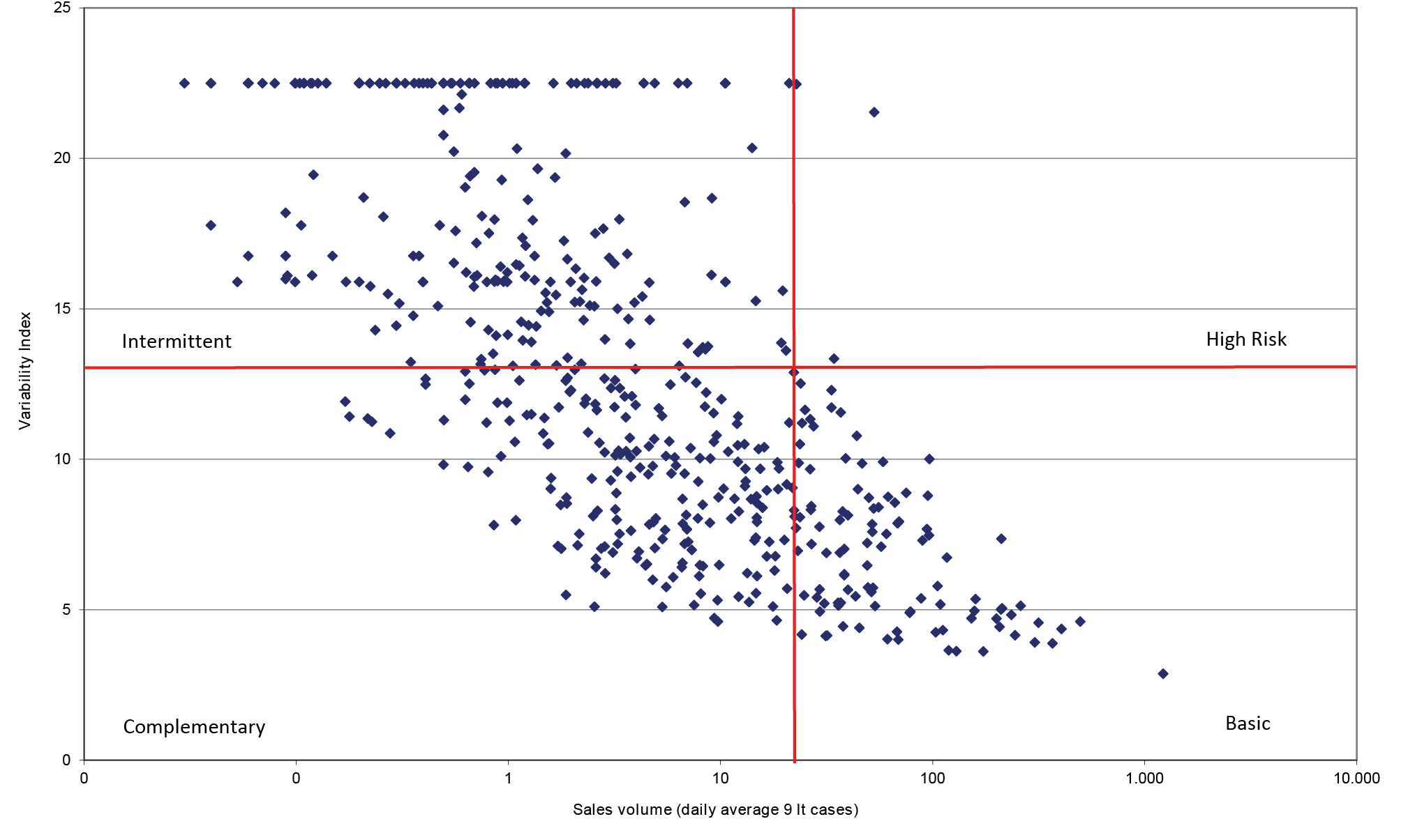
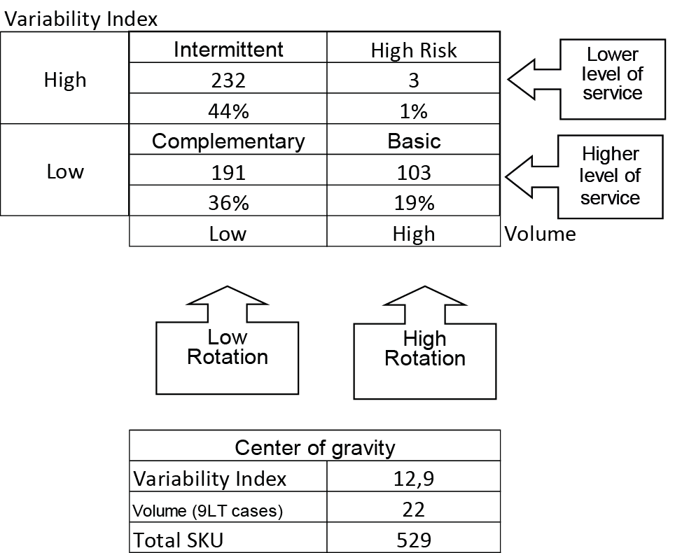
The company was having difficulty implementing a supply chain efficiency strategy that was reflected in the difficulty of meeting delivery promises, very low customer satisfaction and high inventories. With the graphs, the company’s decision makers quickly understood the complexity of the supply chain and the need to reduce it. Several improvement points were recommended.
The company decided to purge products with IV greater than 12 because they increase the complexity of the supply chain; there were 258 SKUs in this condition. Products with IV of 22 were found with one sale in 500 days, with IV of 15 with two sales in 500 days, with IV of 12 with three in 500 days. This low frequency of sales did not make sense for an efficient supply chain strategy oriented to a mass consumer market. Excluding products with IV greater than 12, the new product portfolio had an average variability of 8.
There were 3 high-risk products that in an ABC classification could appear as A products. These are products that will not be sold again and could generate a whip effect in the purchase of raw materials and wine stock. Complementary wines generate complications for the economic bottling lot, and in the case of exports, it is necessary to create stocks of bottled wines without labels.
4.3 Variability of the finished products of Winery V2
The results of the variability of the independent demand for finished products are shown in Figures 7 and 8.
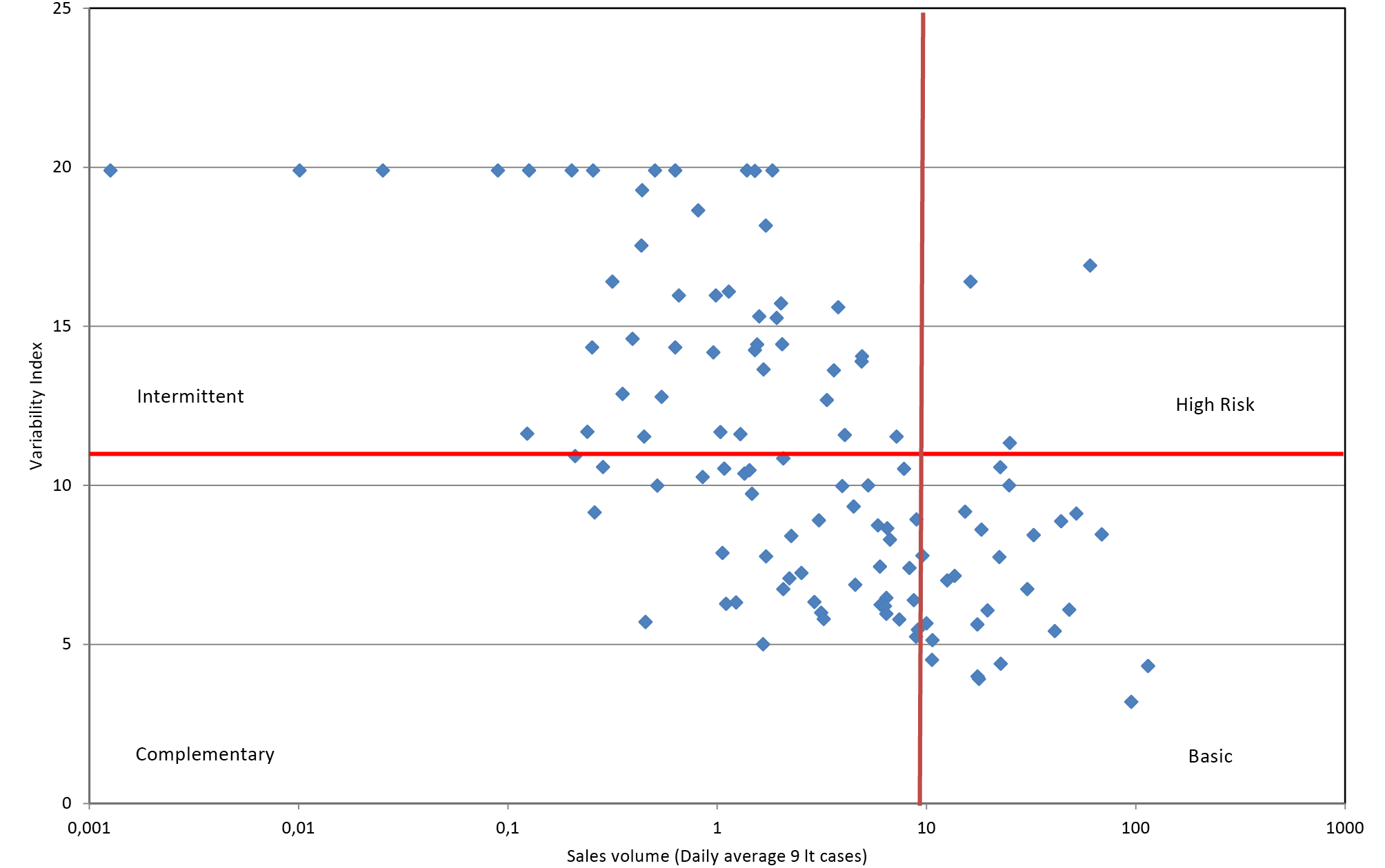
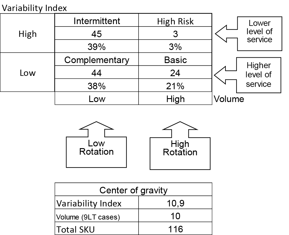
The company was having difficulty implementing the supply chain efficiency strategy which resulted in not being able to make a profit. Despite the fact that this vineyard had better average prices than vineyards A and C.
It had an average IV of 10.94 which is a high IV due to tactical decisions taken from the company with the sale of products with low rotation. It was recommended to purge SKUs with IV > 12 due to low sales frequency and that are contradictory to having an efficient supply chain strategy. The decision makers agreed.
4.4 Variability of the finished products of Winery V3
The results of the variability of independent demand for finished products are shown in Figures 9 and 10.
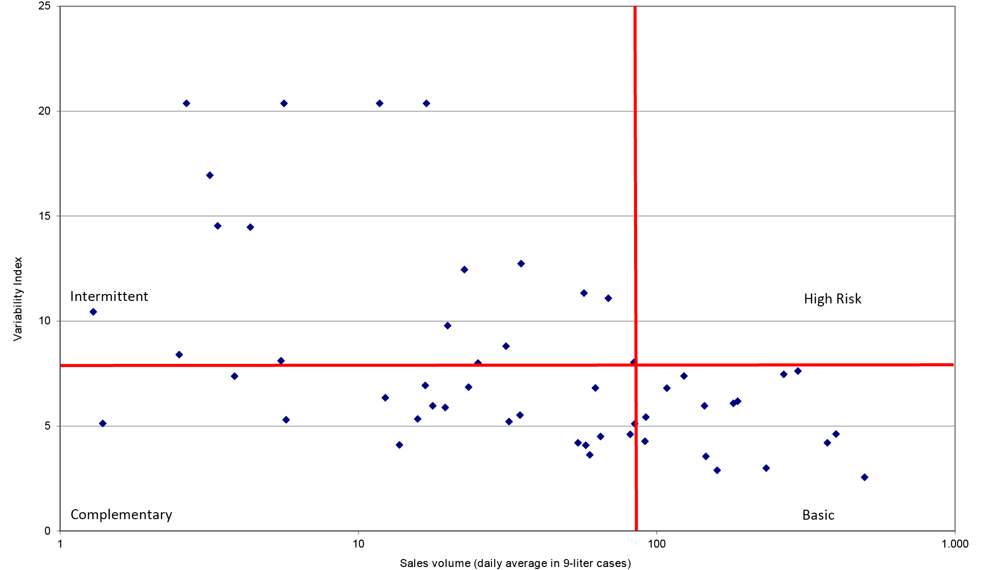
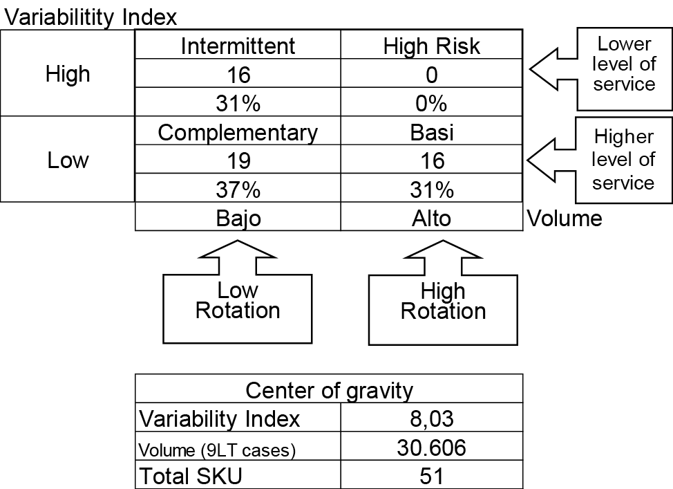
The company has an IV of 8.03, partly due to the lower number of SKUs and tactical decisions made. SKUs with IV > 12 must be purged due to low sales frequency and because they hinder efficient supply chain strategy.
4.5 Variability of finished products ABC of Winery V1
The products with classification A for Vineyard V1 are shown below within the 2x2 matrix format in order to observe the behavior of products that are supposed to have high turnover. The results are shown in figure 11.
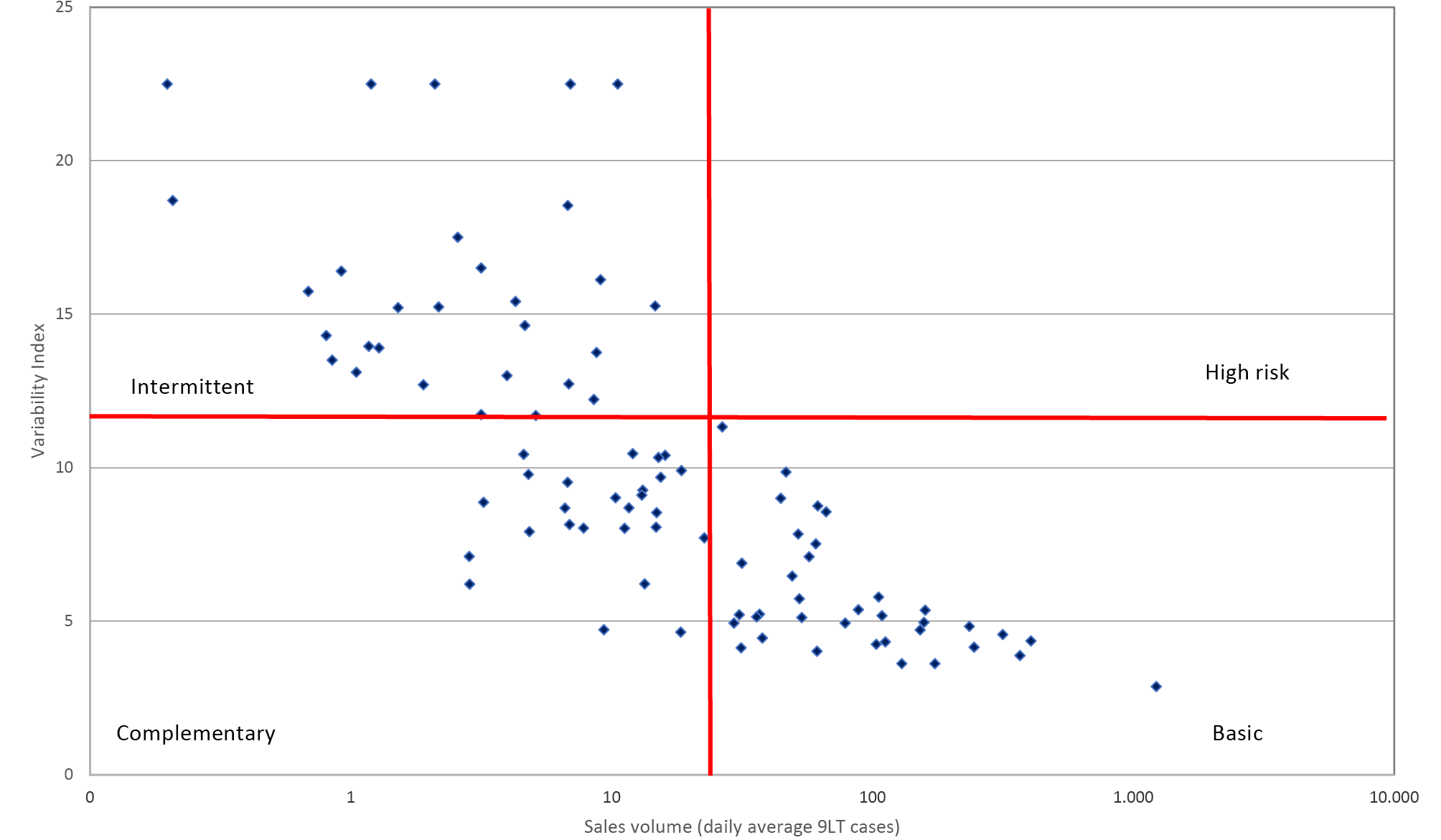
Class A products by definition of the ABC classification should have a higher service level due to their combination of high turnover and high value.
By plotting them in the 2x2 matrix with demand uncertainty we can see that there are weaknesses. Infrequently sold intermittent products are not easy to forecast, to plan, so they should have low service level. But if they have a high value they can be classified as A as we see in Figure 11.
We have product A that are basic (low variability, high average sales) and should have the highest level of service. We have product A that are complementary (low variability, low average sales) and should not have the same resources as the basic ones.
In this case there is no high-risk product (high variability and high average sales), but if there were, the A classification would lead us to produce large quantities of products that will be very difficult to sell, which generates the whip effect with wine and wine inputs.
A comparative summary of the 3 wineries is presented in Table 1.
| Winery | SKU Number | Variability Index | |||||||||||||||||
|---|---|---|---|---|---|---|---|---|---|---|---|---|---|---|---|---|---|---|---|
| V1 | 529 | 12.90 | |||||||||||||||||
| V2 | 116 | 10.94 | |||||||||||||||||
| V3 | 51 | 8.03 | |||||||||||||||||
| Source: Elaborated by the author. | |||||||||||||||||||
We can observe that the three wineries have high variability to have an efficiency strategy. Although demand uncertainty should be low for mass consumption wines, this uncertainty is amplified by planning or tactical decisions in the supply chain: bottling with country labels increases product uncertainty, there were no restrictions on the number of products that could be requested in an order, the incentives to increase export sales led to accepting customer requirements for blends of wines (which were not sold later and whose balances generated problems), requirements for special bottles (which made subsequent supply more complex), decisions on functional silos, etc.
The data collected from the case demonstrate that quantitative theoretical methods are not applied to measure supply chain uncertainty.
The qualitative method by [43,44] is quite reliable and better than the ABC method for tactical decisions. It allows to put a value to the uncertainty by means of the variability index and to be able to compare the complexity with other units. It has a value of variability or uncertainty for each product, which allows to compare it or to know that a product debugging is needed.
The graphical interface has a very high level of user acceptance. In product debugging discussions it was very difficult for anyone to defend products with IV greater than 12. Displaying the variability graphs showed the damage that was done by making the whole supply chain more complex.
You can compare uncertainty levels of different stages of the supply chain such as bottling and winemaking. In other words, uncertainty can be measured by independent demand (sales dispatches) and by dependent demand (production receipts to in-process warehouses).
This classification by demand uncertainty allows more appropriate production and inventory management decisions to be defined (such as demand forecasting methods, inventory policies, etc.), which are beyond the scope of this study. A better level of service and performance should be expected in commodity and complementary products.
It is necessary to incorporate the measurement of the uncertainty of the demand of the supply chain as an indicator of performance of the wine industry. We did not find it in the reviews at a global level carried out such as the studies of [52]. Nor did we find it in reviews on performance indicators in the wine industry in Chile [53]. In reviews on wine industry risk management in market issues only price volatility is studied [54].
In comparison with previous research that has explored strategic and supply-side responses to uncertainty [2,3], this study adds value by focusing on demand uncertainty at the product level and its operational implications. Unlike general process improvement strategies such as Lean Six Sigma [4], which seek to enhance system efficiency, this classification approach allows for product-specific diagnostics and segmentation. This supports differentiated policies for forecasting methods, service levels, and inventory strategies. Furthermore, as demonstrated in [45], the model is adaptable to multiple stages of the wine production chain, including in-process goods and critical inputs such as corks and bottles. Thus, the tool contributes not only to decision-making on finished goods, but also to reducing supply chain complexity as a whole by enabling better tactical and operational planning across multiple inventory categories.
This study shows that current business practice in the wine industry often lacks quantitative methods for measuring supply chain uncertainty, relying instead on the traditional ABC classification and expert judgment. As such, uncertainty is not systematically measured or used to support tactical and operational decision-making.
Through the case analysis of three wineries in Chile´s Central Valley, we found that the quantitative method based on demand uncertainty [43,44] provides a superior classification of products compared to the ABC method. This classification enables more nuanced and appropriate decisions on inventory policy, demand forecasting, and service level differentiation.
The study contributes to bridging the gap between theory and practice by providing a replicable methodology rooted in demand behavior that can be adapted to different stages of the wine supply chain.
Unlike more generic process optimization frameworks, the demand uncertainty matrix provides product-level insights that allows wineries to reduce complexity, align production and bottling strategies, and implement inventory segmentation. These insights offer direct benefits in supply chain performance, customer service, and operational efficiency.
This research is novel given that, it contributes with empirical information in bridging the gap between theory and practice on product classification by uncertainty and in relieving the need for its use for tactical wine supply chain decisions. At the same time, it opens the door to future research to replicate this methodology in other contexts and to investigate the most appropriate production and inventory management decisions based on this product classification.
[1] C. Bopp, R. Jara-Rojas, A. Engler, M. Araya-Alman. How are vineyards management strategies and climate-related conditions affecting economic performance? A case study of Chilean wine grape growers. Wine Economics and Policy 2022;11:61–73. https://doi.org/10.36253/wep-12739.
[2] E. Haddad, P. Aroca, P. Jano, A. Rocha, B. Pimenta. A Bad Year? Climate Variability and the Wine Industry in Chile. Wine Economics and Policy 2020;9:23–35. https://doi.org/10.36253/web-7665.
[3] A. Gilinsky, A. Sen, J. Ford, S.C. de la Torre, S.K. Newton. US Wine Industry Preparedness For Unforeseen Crises And Disasters: An Empirical Test. Wine Economics and Policy 2020;9:6–18. https://doi.org/10.14601/web-8054.
[4] A. Zironi, P. Danese, P. Romano, R. Zironi. A Lean Six Sigma, Industry 4.0 and Circular Economy-driven methodology for wine supply chain process improvement. Wine Economics and Policy 2024;13:75–88. https://doi.org/10.36253/wep-15803.
[5] J. Mula, R. Poler, G.S. García-Sabater, F.C. Lario. Models for production planning under uncertainty: A review. Int J Prod Econ 2006;103:271–85. https://doi.org/10.1016/j.ijpe.2005.09.001.
[6] E. Simangunsong, L.C. Hendry, M. Stevenson. Supply-chain uncertainty: A review and theoretical foundation for future research. Int J Prod Res 2012;50:4493–523. https://doi.org/10.1080/00207543.2011.613864.
[7] R. Bhatnagar, A.S. Sohal. Supply chain competitiveness: measuring the impact of location factors, uncertainty and manufacturing practices. Technovation 2005;25:443–56. https://doi.org/10.1016/j.technovation.2003.09.012.
[8] G.T.M. Hult, C.W. Craighead, D.J. Ketchen. Risk Uncertainty and Supply Chain Decisions: A Real Options Perspective. Decision Sciences 2010;41:435–58. https://doi.org/10.1111/j.1540-5915.2010.00276.x.
[9] Z. Sazvar, M. Zokaee, R. Tavakkoli-Moghaddam, S.A. sadat Salari, S. Nayeri. Designing a sustainable closed-loop pharmaceutical supply chain in a competitive market considering demand uncertainty, manufacturer’s brand and waste management. Ann Oper Res 2022;315:2057–88. https://doi.org/10.1007/s10479-021-03961-0.
[10] A. Bacchetti, N. Saccani. Spare parts classification and demand forecasting for stock control: Investigating the gap between research and practice. Omega (Westport) 2012;40:722–37. https://doi.org/10.1016/j.omega.2011.06.008.
[11] S. Chopra, P. Meindl. Supply Chain Management 7th edition. Boston: Pearson Education Inc.; 2017.
[12] G. Guillén, F.D. Mele, M.J. Bagajewicz, A. Espuña, L. Puigjaner. Multiobjective supply chain design under uncertainty. Chem Eng Sci 2005;60:1535–53. https://doi.org/10.1016/j.ces.2004.10.023.
[13] H. Min, G. Zhou. Supply chain modeling: past, present and future. Comput Ind Eng 2002;43:231–49. https://doi.org/10.1016/S0360-8352(02)00066-9.
[14] M. Bortolini, M. Faccio, F.G. Galizia, M. Gamberi. Push/pull parts production policy optimization in the ato environment. Applied Sciences (Switzerland) 2021;11:6570. https://doi.org/10.3390/app11146570.
[15] A.P. Velasco Acosta, C. Mascle, P. Baptiste. Applicability of Demand-Driven MRP in a complex manufacturing environment. Int J Prod Res 2020;58:4233–45. https://doi.org/10.1080/00207543.2019.1650978.
[16] D. Simchi-Levi, P. Kaminsky, E. Simchi-Levi. Managing the supply chain the definitive guide for the business professional. New York: McGraw Hill; 2004.
[17] G. Merkuryeva, A. Valberga, A. Smirnov. Demand forecasting in pharmaceutical supply chains: A case study. Procedia Comput Sci, vol. 149, Elsevier B.V.; 2019, p. 3–10. https://doi.org/10.1016/j.procs.2019.01.100.
[18] J.G.A.J. Van Der Vorst, A.J.M. Beulens. Identifying sources of uncertainty to generate supply chain redesign strategies. International Journal of Physical Distribution & Logistics Management 2002;32:409–30. https://doi.org/10.1108/09600030210437951.
[19] M. Babagolzadeh, A. Shrestha, B. Abbasi, Y. Zhang, A. Woodhead, A. Zhang. Sustainable cold supply chain management under carbon tax regulation and demand uncertainty. Transp Res D Transp Environ 2020;80:102245. https://doi.org/10.1016/j.trd.2020.102245.
[20] T. Davis. Effective supply chain management. Sloan Manage Rev 1993;34:35–46.
[21] J.Y. Jung, G. Blau, J.F. Pekny, G.V. Reklaitis, D. Eversdyk. A simulation based optimization approach to supply chain management under demand uncertainty. Comput Chem Eng 2004;28:2087–106. https://doi.org/10.1016/j.compchemeng.2004.06.006.
[22] D. Peidro, J. Mula, R. Poler, F.C. Lario. Quantitative models for supply chain planning under uncertainty. Int J Adv Manuf Technol 2009;43:400–20. https://doi.org/10.1007/s00170-008-1715-y.
[23] F.A. de Lima, S. Seuring, P.C. Sauer. A systematic literature review exploring uncertainty management and sustainability outcomes in circular supply chains. Int J Prod Res 2022;60:6013–46. https://doi.org/10.1080/00207543.2021.1976859.
[24] M. Acuna, J. Sessions, R. Zamora, K. Boston, M. Brown, M.R. Ghaffariyan. Methods to manage and optimize forest biomass supply chains: a review. Current Forestry Reports 2019;5:124–41. https://doi.org/10.1007/s40725-019-00093-4.
[25] A. Gupta, C.D. Maranas. Managing demand uncertainty in supply chain planning. Comput Chem Eng 2003;27:1219–27. https://doi.org/10.1016/S0098-1354(03)00048-6.
[26] B. Bilgen, I. Ozkarahan. Strategic tactical and operational production-distribution models: a review. Int J Technology Management 2004;28:151–71. https://doi.org/10.1504/IJTM.2004.005059.
[27] S. Ghosh, M.C. Mandal, A. Ray. Strategic sourcing model for green supply chain management: an insight into automobile manufacturing units in India. Benchmarking: An International Journal 2021;29:3097–132. https://doi.org/10.1108/BIJ-06-2021-0333.
[28] M.S. Fox, M. Barbuceanu, R. Teigen. Agent-oriented supply-chain management. Int J Flexible Manufacturing Systems 2000:81–104. https://doi.org/10.1023/A:1008195614074.
[29] J. Oh, B. Jeong. Tactical supply planning in smart manufacturing supply chain. Robot Comput Integr Manuf 2019;55:217–33. https://doi.org/10.1016/j.rcim.2018.04.003.
[30] J. Saragih, A. Tarigan, E. Frida, J. Wardati, I. Pratama. Supply chain operational capability and supply chain operational performance: Does the supply chain management and supply chain integration matters? Int J Sup Chain Mgt 2020;9:1222–9.
[31] X. Wen, T.M. Choi, S.H. Chung. Fashion retail supply chain management: A review of operational models. Int J Prod Econ 2019;207:34–55. https://doi.org/10.1016/j.ijpe.2018.10.012.
[32] R. Ganeshan, E. Jack, M.J. Magazine, P. Stephens. A taxonomic review of supply chain management research. Quantitative models for supply chain management, Boston: Kluwer Academic; 1999, p. 840–79. https://doi.org/10.1007/978-1-4615-4949-9_27.
[33] S.Y. Sun, M.H. Hsu, W.J. Hwang. The impact of alignment between supply chain strategy and environmental uncertainty on SCM performance. Supply Chain Management 2009;14:201–12. https://doi.org/10.1108/13598540910954548.
[34] A. Kortabarria, U. Apaolaza, A. Lizarralde, I. Amorrortu. Material management without forecasting: From MRP to demand driven MRP. Journal of Industrial Engineering and Management 2018;11:632–50. https://doi.org/10.3926/jiem.2654.
[35] R. Miclo, M. Lauras, F. Fontanili, J. Lamothe, S. Melnyk, S.A. Melnyk. Demand Driven MRP: assessment of a new approach to materials management. Int J Prod Res 2019;57:166–81. https://doi.org/10.1080/00207543.2018.1464230.
[36] S. Cavalieri, M. Garetti, M. MacChi, R. Pinto. A decision-making framework for managing maintenance spare parts. Production Planning and Control 2008;19:379–96. https://doi.org/10.1080/09537280802034471.
[37] T.J. van Kampen, R. Akkerman, D.P. van Donk. SKU classification: A literature review and conceptual framework. Int J Operations and Production Management 2012;32:850–76. https://doi.org/10.1108/01443571211250112.
[38] J.H. Heizer, B. Render. Principles of operations management. Pearson Education; 2003.
[39] F. Liu, N. Ma. Multicriteria ABC inventory classification using the social choice theory. Sustainability (Switzerland) 2020;12. https://doi.org/10.3390/SU12010182.
[40] V. Lukinskiy, V. Lukinskiy, B. Sokolov. Control of inventory dynamics: A survey of special cases for products with low demand. Annu Rev Control 2020;49:306–20. https://doi.org/10.1016/j.arcontrol.2020.04.005.
[41] A.A. Ghobbar, C.H. Friend. Sources of intermittent demand for aircraft spare parts within airline operations. 2002. https://doi.org/10.1016/S0969-6997(01)00054-0.
[42] A.A. Syntetos, J.E. Boylan, J.D. Croston. On the categorization of demand patterns. Journal of the Operational Research Society 2005;56:495–503. https://doi.org/10.1057/palgrave.jors.2601841.
[43] A.J. D’Alessandro, A. Baveja. Divide and conquer: Rohm and Haas’ response to a changing specialty chemicals market. Interfaces (Providence) 2000;30:1–16. https://doi.org/10.1287/inte.30.6.1.11627.
[44] J.H. Chavez. Supply Chain Management. Santiago de Chile: RIL Editores; 2012.
[45] L.A. Camino Cabrejos, J.P. Vargas Norambuena. Medición de Incertidumbre de Demanda de la Cadena de Suministro del Vino. RIVAR 2025;12:154–75. https://doi.org/10.35588/01jbbd18.
[46] M.L. Fisher. What is the Right Supply Chain for Your Product? Harv Bus Rev 1997;75:105–16.
[47] H.L. Lee. Aligning Supply Chain Strategies with Product Uncertainties. 2002. https://doi.org/10.2307/41166135.
[48] M. Abolghasemi, E. Beh, G. Tarr, R. Gerlach. Demand forecasting in supply chain: The impact of demand volatility in the presence of promotion. Comput Ind Eng 2020;142. https://doi.org/10.1016/j.cie.2020.106380.
[49] L. Xie, J. Ma, M. Goh. Supply chain coordination in the presence of uncertain yield and demand. Int J Prod Res 2021;59:4342–58. https://doi.org/10.1080/00207543.2020.1762942.
[50] C. Voss, N. Tsikriktsis, M. Frohlich. Case research in operations management. Int J Operations and Production Management 2002;22:195–219. https://doi.org/10.1108/01443570210414329.
[51] A. Alonso-Ayuso, L.F. Escudero, A. Garín, M.T. Ortuño, G. Pérez, U. Rey, et al. An approach for Strategic Supply Chain Planning under Uncertainty based on Stochastic 0-1 Programming. Journal of Global Optimization 2003;26:97–124. https://doi.org/10.1023/A:1023071216923.
[52] J. Mota, A. Moreira, R. Costa, S. Serrão, V. Pais-Magalhães, C. Costa. Performance indicators to support firm-level decision-making in the wine industry: a systematic literature review. Int J Wine Business Res 2020;33:217–37. https://doi.org/10.1108/IJWBR-06-2020-0027.
[53] L. Valenzuela, S. Maturana. Designing a three-dimensional performance measurement system (SMD3D) for the wine industry: A Chilean example. Agric Syst 2016;142:112–21. https://doi.org/10.1016/j.agsy.2015.11.011.
[54] A. Seccia, F.G. Santeramo, G. Nardone. Risk management in wine industry: A review of the literature. BIO Web Conf 2016;7:03014. https://doi.org/10.1051/bioconf/20160703014.