Analysing Economic Performance of German Wine Estates Across Three Decades - What can we Learn for the Future?
Department of Wine & Beverage Business, Hochschule Geisenheim University, Von-Lade-Straße 1, D-65366 Geisenheim, Germany
Email: AnthonyWilliam.Bennett@hs-gm.de; Simone.Loose@hs-gm.de
*Corresponding author.
Abstract. In recent decades, the German wine market has undergone significant structural changes due to intensifying competition and shifting consumption patterns. Increased imports and declining exports have pressured German wine estates to adapt for survival. The study explores these long-term trends and structural changes in German wine estates, focusing on those marketing bottled wine. It aims to understand how these businesses have adapted to economic pressures in a highly competitive market from 1993 to 2020, using business panel data and regression analysis for 16 key performance indicators (KPIs). At first (until the financial crisis of 2008) estates benefitted from mechanisation and economies of scale, leading to a significant reduction in labour hours per hectare and moderate increases in wine prices, improving labour productivity and profitability. However, yields declined due to a shift towards lower-yield grape varieties in response to market demand. From 2009 onward, rising labour and material costs as well as stagnating yields started eroding profitability gains, leading to an overall stagnation of long-term profitability. When observing differences in developments between size groups, large wine estates experienced a considerably sharper increase in costs per ha than small to medium sized wine estates, from 2009 onward. Nonetheless, this could be counterbalanced by large wine estates also generating significantly higher productivity increases in the same time period, resulting in a significant increase in profitability for large wine estates from 2009 onward, while small to medium sized wine estates stagnated.
Keywords: key-performance-indicators, business structure, long-term trends, economic crisis, economies of scale.
Index
1.1. The Position of Wine Estates within the German Wine Sector
2. Expectations For Economic Development of Wine Estates
2.1. Overall framework of economic performance
2.2.2. Labour per Hectare and Workforce Composition
2.2.3. Investments per ha and Fixed Assets
2.3.2. Area Productivity and Labour Productivity
2.5. Potential changes of path within the assessed time period
4.1.2. Investments per Hectare and Fixed Assets per Hectare
4.1.3. Labour per Hectare and Workforce Composition
4.2.2. Area Productivity and Labour Productivity
4.3.2. Operational result per hectare
4.3.3. Return on Sales and Equity
5.1. Economic development in phase 1 – prior the financial crisis
5.2. Economic development in phase 2 – after the financial crisis
5.3. Limitations and Future Research
Over the past decades, international wine markets have changed fundamentally and increased internationalisation [1,2]. In a global context, Germany is a medium-sized wine producer and major wine importer [2]. Saturated domestic wine consumption, declining exports, and increasing imports from a highly competitive global bulk wine market have resulted in intense price competition for German wine producers [3,4].
To ensure sustainable long-term survival, various types of wine producers have been driven to adapt. Much like the agricultural sector as a whole, the wine industry has undergone structural change and increased concentration, with wine prices experiencing only marginal growth [5]. This long-term process of consolidation has also been observed in both the German and international agricultural sectors [6,7]. The current economic crisis and significant cost pressures present major challenges for businesses within the wine sector [8].
It is of great interest to understand how wine estates have responded and adapted to competitive market conditions in the past. Gaining insight into existing long-term trends and survival strategies from the past will be invaluable for addressing the present and future challenging conditions [9]. In this context, this paper examines developmental processes using a unique data set of long-term business data from German wine estates, spanning nearly three decades, from 1993 to 2020. The key findings derived from analysing structural changes can provide a deeper understanding of how wine estates have adjusted over time, while also offering potential recommendations for policymakers and wine estates to achieve future economic success.
1.1. The Position of Wine Estates within the German Wine Sector
The German wine market is highly competitive. Wine consumption remained relatively stable until around 2012, after which it began to decline, with a brief but strong recovery during the COVID-19 pandemic [10]. Within this market, German wine holds a significant, yet recently diminishing, market share, decreasing to 44% in 2022 in terms of purchase volume [5,11]. The declining reach of German wine is evident, with the percentage of German households purchasing domestic wine falling from 46.3% in 2004 to 35.9% in 2023. [10].
Globally, Germany ranks among the largest wine importers, with a significant share of these imports comprising bulk wine priced around €0.80 per litre, which is bottled domestically by large, efficient co-packers [2]. After peaking at 3.0 million hectolitres in the 1980s, German wine exports have steadily declined, hitting a historic low of under 1.0 million hectolitres in 2020, with only modest recovery following the post-COVID period and the removal of US wine tariffs. The combination of strong import competition, falling exports, and a gradually declining domestic consumption creates a highly competitive market environment with intense price pressure [12].
Wine estates account for around 27% of the total volume of German wine sold domestically [4]. The approximately 7,000 estates typically operate fully integrated supply chains, growing grapes, producing, bottling, and marketing their own wine. Recently, some estates have begun purchasing bulk wine or grapes to market under their own brand, competing with bottlers and cooperatives for retail space. Predominantly family-owned SMEs, wine estates focus heavily on direct-to-consumer sales, with cellar-door sales playing a key role in regional wine tourism [4,13]. Unlike bottlers or cooperatives, wine estates manage the entire supply chain, making them the least specialised, as family members often develop expertise across multiple areas of production and business management. The fragmented nature of wine production, price competition from imports, and the dominance of large food retailers create a highly competitive market, where most producers, including estates, are price-takers, with only a few differentiating through strong branding.
Wine estates, confronted with this highly competitive environment, have been compelled to adapt their business strategies in various ways in order to ensure survival. This study seeks to analyse and explore the economic and structural changes that German wine estates have undergone, with the aim of sustaining their operations in the long term. Expectations regarding the development of business indicators are drawn from agricultural economics and existing research on the economic evolution of wine businesses.
The long-term development of a total of 16 business factors and key performance indicators (KPIs) are empirically analysed for a sample of wine estates participating in the Geisenheim Business Analysis, based on their balance sheets and income statements over a period of 28 years. In line with research in agricultural economics, the development of these KPIs is examined for potential structural breaks and shifts in trajectory, particularly around the 2008 financial crisis. Additionally, developmental variations of different size groups (small, medium and large) were analysed separately, to gain a deeper understanding if wine estates of different sizes developed homogeneously, or if some size groups were able to develop and adapt to market changes more successfully than others.
2. Expectations For Economic Development of Wine Estates
2.1. Overall framework of economic performance
This study builds on the economic sustainability framework developed by Bennett & Loose [14], with minor modifications (Figure 1). The framework organises economic input factors and Key Performance Indicators (KPIs) into three tiers. These key figures from controlling can, by definition, be derived from one another and categorized into three tiers. The key figures in Tier 2 are ratios of the key figures from Tier 1. Similarly, KPIs in tier 3 further aggregate KPIs from tiers 1 and 2.
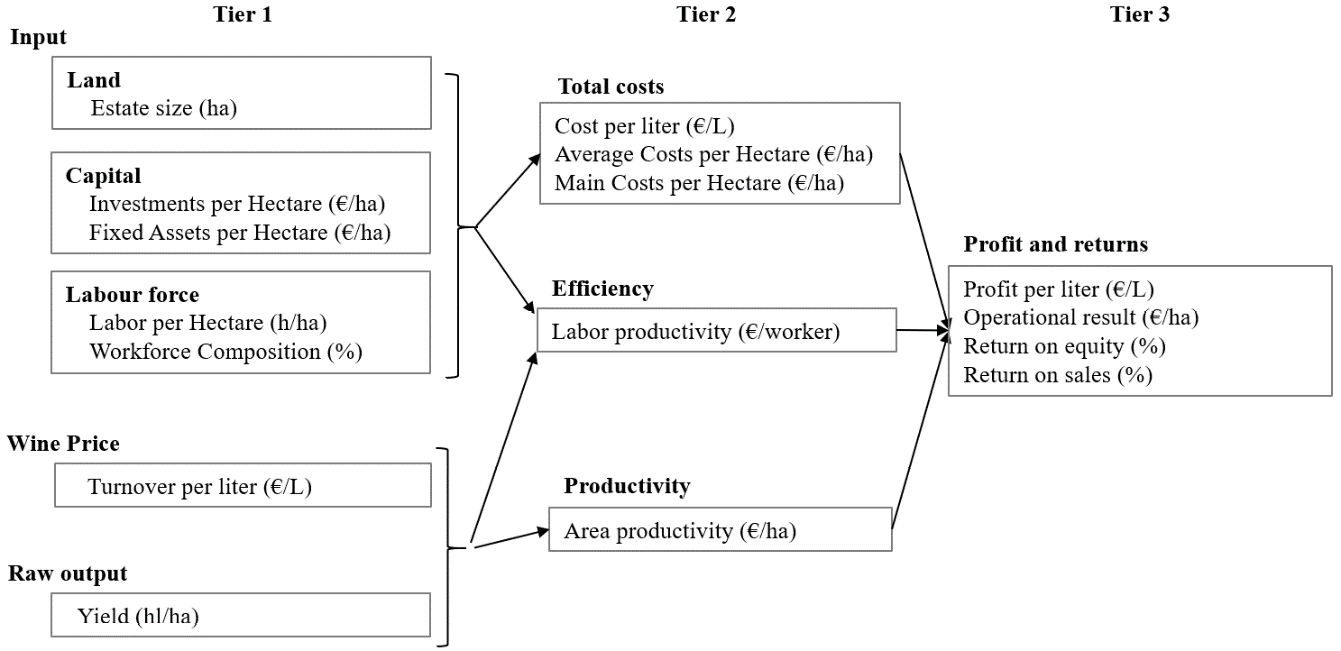
Tier 1 includes traditional agricultural economics input factors such as land, labour (including workforce composition), and capital. It covers the raw output generated by these factors, represented as wine yield per hectare, and its external market valuation, represented as turnover per hectare. This paper builds on previous research by also examining investments, fixed asset structures, and workforce composition within wine estates.
Tier 2 aggregates KPIs from Tier 1, focusing on cost, efficiency, and productivity. Cost per litre considers total costs, including family wages, relative to production volume, while cost per hectare measures costs in relation to estate size. Labour productivity is defined as turnover per worker, and area productivity as turnover per hectare. Although previous studies have examined area and labour productivity, long-term cost trends in the wine estate sector, as analysed here, remain underexplored.
Tier 3 represents the highest level of aggregation. Profit per litre reflects the surplus after accounting for price and cost per unit, while the operational result measures the surplus per hectare. The operational result per hectare includes an imputed family wage, which ensures a fair remuneration for family members working within the wine estate, making it a key indicator of economic sustainability in this framework [14]. Return on equity and sales are calculated from profit relative to total equity and turnover. While profitability has been studied in agricultural and wine economics, long-term trends in profit per litre remain largely unexplored.
The following subsections outline expectations for the long-term development of these KPIs, based on existing literature in agricultural and wine economics. For areas where research is limited, statistical data and relevant considerations are used to establish expectations.
In recent decades, the agricultural sector has seen significant consolidation across numerous countries [6,9,15,16]. Increased globalisation has heightened competition in international agriculture, leading to substantial restructuring [9]. In the US, average farm size expanded dramatically from the 1940s to the 1980s, with the number of large farms more than doubling between 1987 and 2017 [6]. In Germany, the number of agricultural businesses halved between 1995 and 2020, while average business size grew by 62% [17]. These changes are often attributed to efficiency gains through economies of scale [18,19].
In the wine sector, studies indicate that larger businesses tend to be more efficient, with size-related performance benefits attributed to the greater viability of mechanisation, such as the use of grape harvesters [20–22]. Research on consolidation in the wine industry has primarily focused on cooperatives, large companies, and distributors, especially in countries like Italy and Spain [20,23–25]. However, there is limited research on the concentration of family-run wine estates that primarily market their own bottled wine. The trend of consolidation and increasing business size in agriculture is anticipated to continue in the wine sector, likely leading to a gradual increase in the average size of wine estates.
2.2.2. Labour per Hectare and Workforce Composition
Annual Work Units
The agricultural industry has seen several labour-related changes in recent years. Rising opportunity costs for farm labour, due to higher wages in non-farm sectors, have driven the development of labour-saving technologies [6,26]. Larger farm sizes make it more viable to adopt these technologies by investing in large machinery, resulting in efficiency gains [21,27]. In Germany, despite increasing farm sizes, the Annual Work Units (AWU) per farm halved from 1990 to 2020 [28]. Although no data on AWU trends for wine estates in Germany is currently available, a reduction in labour per hectare required is anticipated, based on developments of the broader agricultural sector.
Workforce Structure
In agriculture, workforce structures have shifted despite rising business sizes. From 1995 to 2020, the number of family workers per business remained stable, while growth was managed through a significant rise in both permanent and temporary employees [28]. Similar trends are expected in the wine sector, which also relies heavily on family and temporary workers. However, since wine estates manage the entire supply chain, growth leads to more specialised labour needs, including management and administrative roles, making an increase in permanent employees likely [14].
2.2.3. Investments per ha and Fixed Assets
The adoption of labour-saving technologies, increased mechanisation (as discussed in sections 2.2.1 and 2.2.2), and the potential expansion of productive capacity through business growth require capital investment, leading to an anticipated rise in average investments per hectare over time [6,29]. These investments are expected to result in increased technological assets, machinery, and vehicle fleets necessary for the supply-chain processes in viticulture and wine production. In contrast, expansion in sales and marketing typically does not require costly machinery but is reflected in increased salaries as part of variable costs.
The demand for German wine has been visibly declining, reflected in a shrinking market share, reduced domestic consumption, and falling exports [11,12]. Combined with price competition from imports, this forces German producers to compete for the remaining demand, creating a highly competitive market with significant price pressure [12]. Given this weakening bargaining power, producers are unlikely to achieve substantial increases in real prices over the observed period.
In recent decades, agricultural businesses have seen increased productivity due to improvements in plant material and fertilisation, leading to higher yields across the sector [30–32]. However, the conditions for wine and grape production differ significantly. The wine sector is highly diverse, with products varying by grape varieties, appellations, and price segments. Additionally, it is heavily regulated, with strict yield limits per hectare to ensure quality and comply with regional regulations.
In Germany, there has been a shift towards market preferences by replacing high-yield grape varieties from the 1970s with more traditional, lower-yield varieties, such as Riesling, Pinot Gris, and Pinot Noir [33]. Data on average wine must yields indicate a long-term decline in volume [34]. As a result, no significant increase in long-term yield development is expected in the wine sector, unlike the trends seen in broader agriculture.
The cost of agricultural input products in Germany has steadily risen over recent decades [35]. Data show that average material costs per hectare for German wineries increased by 27% between the 2006/07 and 2021/22 agricultural years [36,37]. Labour costs, driven largely by the introduction of minimum wages in 2015, rose even more sharply, increasing by 106% over the same period [36,37]. After high inflation rates following German reunification, interest rates were initially high in the early 1990s but steadily declined to low levels by the mid-1990s, with central banks imposing negative rates after the financial crisis, keeping financing costs very low until around 2021[38].
This variation in cost growth over time indicates a shift in the composition of main costs, with labour and material costs rising, while financing costs decreased. The sharp rise in labour costs post-minimum wage introduction suggests a temporary acceleration in overall cost increases.
2.3.2. Area Productivity and Labour Productivity
The adoption of labour-saving technologies and specialisation, as outlined in section 2.2.2, along with improvements in planting material and fertilisation, as discussed in section 2.2.5, have contributed to notable productivity gains in the agricultural sector globally [26,29,32]. In particular, increases in land productivity (output per hectare) and labour productivity (output per annual work unit, AWU) have been observed. In Germany, area productivity (measured in €/ha) has risen by 72% over two decades, from 2001/02 to 2021/22 [37].
However, the wine sector is less likely to benefit to the same extent from improvements in planting material and fertilisation. Instead, the primary drivers of productivity gains in this industry are increased mechanisation and the adoption of labour-saving technologies. Wine estates must reach a certain scale to fully benefit from mechanisation, such as grape harvesting or woodcutting machinery [21]. As a result, the efficiency of larger wine businesses, due to reduced labour requirements per unit of output, outperforms smaller ones [20,27].
An additional benefit of increasing average business sizes is the effect of specialisation, particularly relevant for wine estates operating across all stages of the supply chain. In smaller operations, a family of two typically manages viticulture, winemaking, administration, marketing, and sales, which limits specialisation and creates time conflicts. For example, sales and marketing often receive less attention during busy periods such as plant protection or harvest seasons. The division of labour, with tasks allocated to specialised roles, has been shown to increase economic efficiency and labour productivity [39–41].
In summary, the productivity gains seen in the agricultural sector, combined with anticipated improvements from technological advancements and specialisation due to larger business sizes, suggest rising area and labour productivity over time.
Return on Sales and Return on Equity
Return on sales (ROS) and return on equity (ROE) for German agricultural businesses have fluctuated significantly over the past two decades, averaging 2.7% and 1.3% respectively from 2001/02 to 2021/22 [37]. This aligns with stable ROS and ROE values observed in agricultural businesses across several European countries between 2009 and 2015, though some were negatively impacted by the global financial crisis until around 2010 [42].
Official statistics for German wine estates, including those producing high shares of bulk wine, suggest a stronger performance than agriculture overall. Wine estates nearly doubled their average ROS from 5.97% in 2006/07 to 11.5% in 2021/22, while average ROE rose from 2.86% to 7% over the same period [43]. Given these trends, an increase in both ROS and ROE is anticipated for wine estates in this data set, specifically focusing on bottled wine.
Operational result and profit per litre
The average operational result of German wine estates increased by 12.9% from 2006/07 to 2021/22, though this does not account for an imputed family wage for estate owners [43]. Over the same period, average profit per hectare grew by 20.3% [43]. Long-term trends in profit per litre for German wine estates remain unexplored.
Given the expected decrease in yield (section 2.2.5), only approximate conclusions can be drawn about its impact on profit per hectare. However, a slight increase in profit per litre may still result from efficiency gains from larger estate sizes. The average operational result per hectare is expected to continue increasing in line with historical trends.
2.5. Potential changes of path within the assessed time period
Major economic events can create structural breaks or shifts in developmental paths for various sectors. The literature has identified the 2008 financial crisis, triggered by the sub-prime mortgage collapse, as such an event with significant implications for the agricultural sector [44,45]. Several studies confirm the long-lasting impacts of the financial crisis on both economies and societies, including persistent effects on economic systems and growth capacity [46], slower recovery in regional areas [47], and long-term shifts in political sentiment [48].
The pronounced impact of the global financial crisis has been consistently highlighted in agricultural economics. When examining agricultural developments over periods that include the 2008 financial crisis, structural breaks and functional changes in the sector were evident post-2008 [45,49–52]. As this study spans both the pre- and post-crisis period, it will consider potential changes in developmental trajectories by dividing the analysis into two phases: before and after 2008.
Data was sourced from the Geisenheim Business Analysis [14,53]. It comprises internal business data from participating wine estates. Due to the voluntary nature of participation, a potential self-selection bias in the sample could limit its representativeness for German wine estates in general. The sample includes only wine estates where bottled wine constitutes at least 80% of total revenue. Wine estates primarily selling bulk wine or grapes were excluded, as they cover only the initial stages of the supply chain and have a fundamentally different cost structure.
The initial sample size was 106 wine estates in 1993, shortly after the project’s inception. A gradual expansion saw the sample grow to 182 estates by 1999. However, a change in project leadership in 1999 caused a drop to 112 wine estates in 2000. From that point, the sample size gradually increased over the next decade, reaching 311 wine estates in 2010. Since then, the sample size has stabilised at around 300 wine estates per year. A slight reduction in the most recent year analysed (2020) occurred due to delays in data preparation and provision by tax consultants. A detailed distribution of the sample sizes for each year can be found in Table 4 (see Appendix A, Table 4).
The Geisenheim Business Analysis is a panel study of wine estates, with participation varying over time. On average, wine estates remain in the sample for seven years, though some have participated throughout the entire observation period. This exploratory analysis, spanning 28 years, does not account for panel or individual business effects; instead, each estate is treated as a separate observation for each year.
In 2017, all historical data was transferred into a unified data management system. This process involved correcting obvious data entry errors, standardising the data to a single currency (the Euro, replacing the Deutsche Mark as of 01.01.2002), and adjusting the data to net values excluding VAT. Extreme outliers (defined as values more than 2.5 standard deviations from the mean) were removed using RStudio.
For 16 Key Performance Indicators (KPIs), yearly averages across all businesses were calculated over the 28-year period from 1993 to 2020. These were graphed in Excel, and linear trend lines were fitted. A visual inspection of the graphs and trend lines guided the decision to divide the linear regressions into two phases. Graphs that showed clear changes in trend around 2008/09 (coinciding with the global financial crisis) were split into two phases: 1993–2008 (Phase 1) and 2009–2020 (Phase 2). Regression coefficients were calculated for both the overall period and/or the two separate phases. For KPIs influenced by earlier tiers of the economic framework, these were also divided into two phases to ensure consistency. Dividing the KPIs into phases allowed the trend lines to better align with the observed data, as well as a more accurate and nuanced understanding of its implications. Since this is an exploratory analysis, with the focus being on investigating the long-term developments of said KPIs, significance tests between the two phases were not conducted, as such tests would exceed the scope of this paper [44,45,50–52,54].
To evaluate whether size groups developed homogeneously, wine estates were divided into terciles based on vineyard area, representing small, medium-sized, and large estates. Since the average wine estate expands over time, the relative business size of these three groups is not static but increases accordingly (see Appendix B, Figure 18).
Regression analysis was performed using IBM® SPSS® (Statistical Package for Social Sciences). Adjustments for inflation were calculated using data from the German Federal Office of Statistics, with 1993 as the base year. Although the residuals were not perfectly normal, the increased sample size (above n=100) was sufficient for the Central Limit Theorem to apply. This ensures that the sampling distribution of the regression coefficients is approximately normal, allowing for valid interpretation of standard confidence intervals and hypothesis tests [55,56].
Additionally, since the assumption of homoscedasticity was not fully met, residual plots were inspected, and extreme outliers were removed to reduce the influence of individual data points on model fit and variance, indicating that the impact on the model was limited. The overall pattern of results remained stable, suggesting that the core findings are robust to minor violations of this assumption [57].
To investigate potential differences in development across business sizes, regressions were performed separately for each tertile, with confidence intervals of the regression coefficients analysed to identify statistically significant variations. Due to space constraints, these differences are presented in tables in the appendix only if significant differences were observed between at least two tertile groups.
The following section presents the results of the linear regression for each tier, accompanied by graphical visualisations of the long-term development of the KPIs over the 28-year period. The graphs display the starting value in 1993, the end value in 2020, and the linear trend across the full period, or two separate slopes for the distinct phases (1993–2008 and 2009–2020).
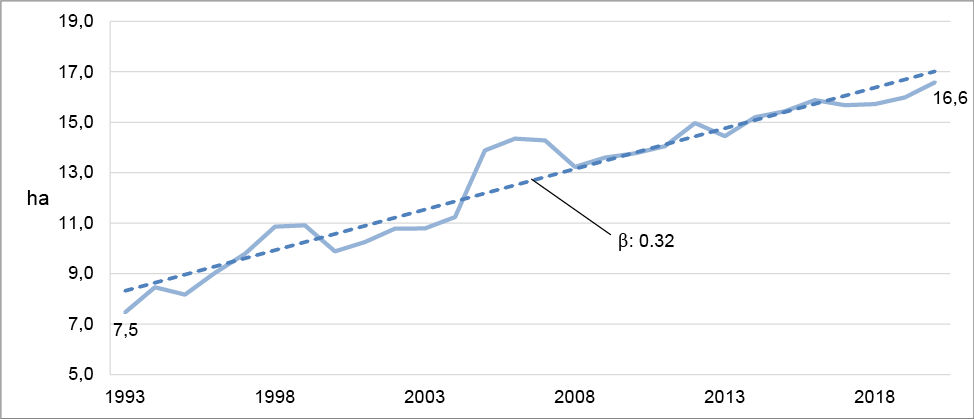
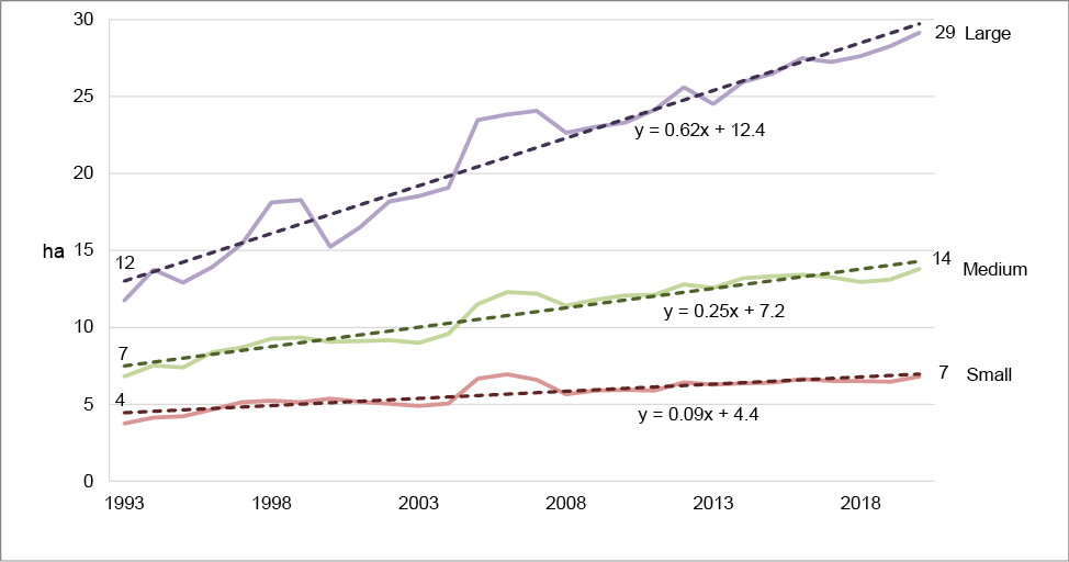
The average size of wine estates exhibited consistent and highly significant growth over the 28-year period, more than doubling from 7.5 hectares in 1993 to 16.6 hectares in 2020 (Figure 2, Table 1). As shown by the slope in Table 1, wine estates expanded by an average of 0.3 hectares per year. The three size groups exhibited significantly different growth trajectories. While large wine estates expanded by 0.62 hectares per year, small estates grew by only 0.09 hectares annually (Appendix C, Table 5).
| Variable | Total timespan (1993 - 2020) | Phase 1 (1993 - 2008) | Phase 2 (2009 - 2020) | |||||||||
|---|---|---|---|---|---|---|---|---|---|---|---|---|
| Coefficients | Corrected R² | Coefficients | Corrected R² | Coefficients | Corrected R² | |||||||
| Coefficient | T-value | p-value | Coefficient | T-value | p-value | Coefficient | T-value | p-value | ||||
| Business Size (ha) | 0.32 | 18.17 | <0.001 | 0.92 | - | - | - | - | - | - | - | - |
| Investments per ha (€/ha) | ||||||||||||
| nominal | 20.63 | 1.50 | 0.145 | 0.04 | - | - | - | - | - | - | - | - |
| real | -29,75 | -2,62 | <0.05 | 0,18 | - | - | - | - | - | - | - | - |
| Fixed Assets per ha (€/ha, nominal) | ||||||||||||
| Viticultural area | -321.43 | -6.84 | <0.001 | 0.63 | -334.07 | -2.17 | <0.05 | 0.21 | -125.50 | -1.70 | 0.118 | 0.14 |
| Buildings for agricultural use | 102.56 | 2.38 | <0.05 | 0.15 | - | - | - | - | - | - | - | - |
| Technological assets and machines | 36.31 | 2.97 | <0.01 | 0.22 | - | - | - | - | - | - | - | - |
| Vehicle fleet | -9.62 | -3.07 | <0.01 | 0.24 | - | - | - | - | - | - | - | - |
| Labour per hectare (h/ha) | -14.59 | -9.18 | <0.001 | 0.76 | -25.51 | -7.27 | <0.001 | 0.79 | -0.77 | -0.41 | 0.687 | -0.07 |
| Workforce composition | ||||||||||||
| % Family workers | -0.61 | -14.00 | <0.001 | 0.88 | - | - | - | - | - | - | - | - |
| % Full-time employees | 0.85 | 34.58 | <0.001 | 0.98 | - | - | - | - | - | - | - | - |
| % Temporary employees | -0.20 | -5.34 | <0.001 | 0.51 | - | - | - | - | - | - | - | - |
| Turnover per Litre (€/L) | ||||||||||||
| nominal | 0.06 | 7.06 | <0.001 | 0.65 | 0.05 | 2.14 | 0.054 | 0.22 | 0.12 | 5.43 | <0.001 | 0.70 |
| real | 0.00 | -0.14 | 0.887 | -0.04 | 0.00 | -0.18 | 0.862 | -0.08 | 0.04 | 2.73 | <0.05 | 0.35 |
| Yield (hl/ha) | -0.63 | -2.62 | <0.05 | 0.18 | -1.21 | -1.91 | 0.078 | 0.16 | -0.13 | -0.17 | 0.867 | -0.09 |
4.1.2. Investments per Hectare and Fixed Assets per Hectare
Major investments in buildings, machinery, or cellar equipment are infrequent for wine estates, as buildings can last over 30 years and tractors for more than 10 years. Consequently, it is not surprising that average investments per hectare fluctuate significantly over time (Figure 3). The nominal average increase in investments of €21 per hectare was non-significant (Table 1), indicating that they remained relatively constant over time. However, when adjusted for inflation, real investments per hectare show a significant downward trend, with a reduction of €30 per hectare per year on average (Table 1). Generally nominal investment increased with business size, but due to high variance this difference was not statistically significant.
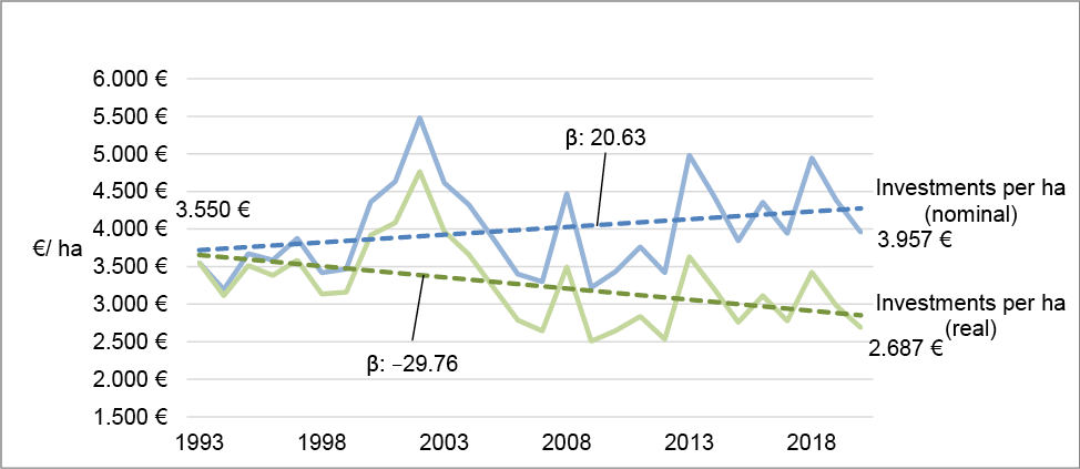
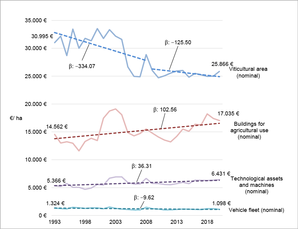
Figure 4 shows the long-term development of major asset categories of wine estates, viticultural area, buildings, technological assets and machines as well as vehicles. The average value of land used for viticulture per hectare fluctuates significantly (Figure 3). Values were higher before 2008, followed by a sharp decline after 2010, with minimal change through to 2020. Analysing both periods separately shows a significant reduction of €334.10 per hectare during 1993 to 2008, while no significant linear trend is observed from 2009 to 2020 (Table 1). The decrease around 2010 may be linked to the reassessment of land value as loan collateral following the financial crisis, when banks increased collateral requirements to mitigate risk. Another possible explanation is a decline in the marginal productivity of land, which is likely associated with a decrease in land value.
The nominal value of viticultural land shows a consistent decline over the entire time span for small wine estates, whereas no such trend is evident for large estates. For medium-sized estates, land values decrease significantly in the first period but recover in the second. This pattern may indicate that larger businesses successfully preserved the marginal productivity of their land (Appendix C, Table 6).
The average value of agricultural buildings per hectare increased significantly from 1993 to 2020 (Table 1). A notable peak between 2001 and 2004 can be attributed to both changes in the sample and a surge in the construction of vinotheques, which tapered off with the financial crisis. After recovering from the crisis, building investments appeared to rise again from 2011 onwards. Over the entire period, building asset values increased due to both a rise in value per hectare and an expansion in hectare size.
Technological assets and machinery values showed modest growth during the observation period (Figure 4). with the average value rising from €5,366 per hectare in 1993 to €6,431 per hectare in 2020. As wine estates expanded by approximately nine hectares during this time (Figure 2), this indicates an overall increase in the total value of technological equipment.
Conversely, the average value of vehicle fleets decreased from €1,324 per hectare in 1993 to €1,098 per hectare in 2020 (Table 1). This reduction may reflect economies of scale, as wine estates ranging from 7.5 to 16.6 hectares (Figure 2) typically require a similar vehicle fleet, with substantial expansion in fleet size only necessary for estates of 20 hectares or more.
Per hectare, smaller and medium-sized wine estates tended to invest more in agricultural buildings, technological assets, machinery, and vehicle fleets, which may be linked to economies of scale. However, due to high variance, these differences were not statistically significant.
4.1.3. Labour per Hectare and Workforce Composition
The development of labour hours per hectare is clearly divided into two distinct phases. From 1993 to 2008, labour hours decreased significantly by 25.5 hours per hectare (Table 1 and Figure 5). However, from 2009 onwards, average labour hours plateaued, fluctuating slightly around 800 hours per hectare (Figure 5, Table 1). It is important to note that the hours per hectare encompass all activities within the wine estate, including viticulture, cellar work, management, and sales/marketing.
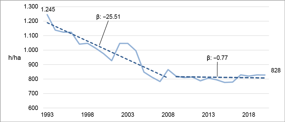
The first phase reflects the widespread adoption of mechanical harvesters, which significantly reduced the manual labour required during harvest. Once these harvesters were universally implemented, no comparable progress in mechanisation followed.
In the last 15 years of the period analysed, three key developments influenced labour demand. First, increased market competition after the financial crisis led wine estates to invest more in sales and marketing personnel. Second, a growing proportion of organic wine estates and a greater commitment to environmentally sustainable practices increased labour requirements in viticulture. Finally, rising administrative demands over time added to the hours needed for general managerial tasks within the wine estates. These three developments have likely counteracted any additional time savings from economies of scale.
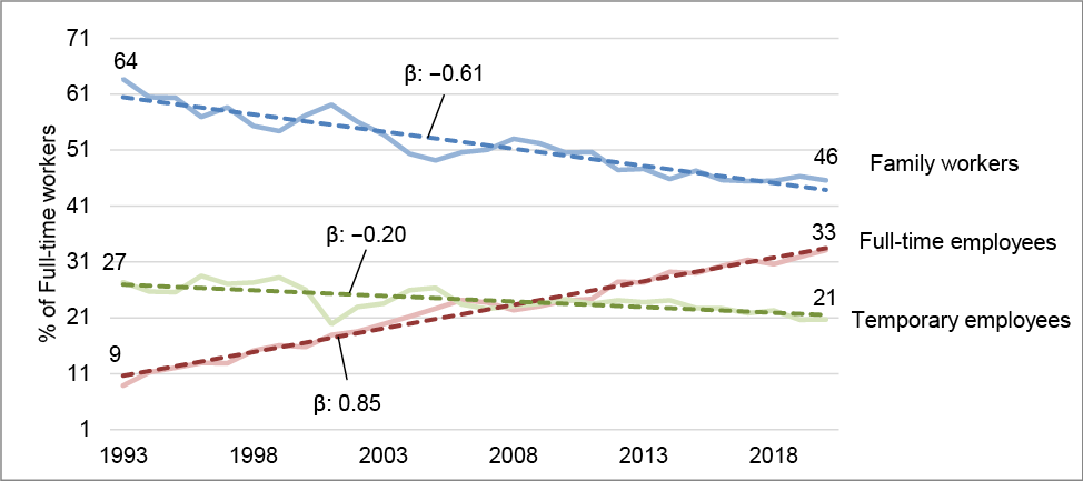
There was a consistent shift in the workforce structure over time. The relative share of family workers decreased significantly by 18%, from 64% in 1993 to 46% in 2020 (Figure 6). Conversely, the proportion of full-time employees moved from 9% in 1993 to 33% in 2020, a highly significant change. Temporary employees, however, gradually declined on a relative basis, from 27% in 1993 to 21% in 2020 (Table 1). These results suggest that wine estates expanded by employing more full-time staff, reflecting a greater need for skilled labour over temporary assistance. The relative number of full-time employees increased significantly more in large wine estates, highlighting their capacity for specialization (Appendix C, Table 5). Interestingly, there were no significant differences in the overall decline in labour per hectare over time, although the negative tendency was stronger for smaller wine estates.
Turnover per litre fluctuates due to annual yield variations. After strong harvests, wine estates often need to sell more bulk wine at lower prices, as they cannot bottle and market all of it at higher prices. Despite these fluctuations, there appears to be a structural break in turnover per litre around the 2008 economic crisis.
In the period leading up to 2008, nominal turnover per litre grew slowly, though the increase was only marginally statistically significant (Figure 7, Table 1). After the financial crisis, while prices dipped for a few years, a stronger growth trend emerged during the recovery. From 2008 to 2020, nominal turnover per litre increased significantly (Table 1). The three size groups did not exhibit significant differences in the development of nominal turnover over time.
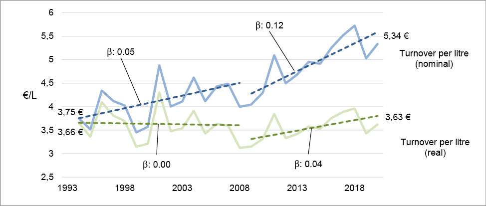
When adjusted for inflation, real turnover per litre remained stagnant in the first phase and grew modestly by €0.04 per litre annually from 2008 to 2020. However, due to the lower starting point post-2008, real turnover per litre showed little change over 28 years (Figure 7). This suggests that, when adjusted for inflation, average prices of wine sold by estates focused on bottled wine have remained relatively stable over the past 30 years.
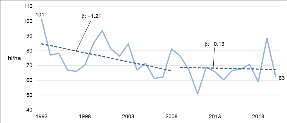
As expected, average yields fluctuated significantly over the observed years due to variations in annual weather conditions (Figure 8). While there is no obvious clear demarcation, the graph suggests two distinct phases: a decline in yield during the first phase and stagnation in the second. Using 2008 as the cut-off point, consistent with the rest of the analysis, the first phase shows an average yield decline of 1.21 hl per hectare, which is marginally statistically significant. In the second phase (2009–2020), the slight reduction of 0.13 hl per hectare is not statistically significant (Figure 8, Table 1). The development of yield over time did not differ significantly among the three size groups.
Cost per Litre
Most costs for a wine estate are independent of yield. Due to weather-related yield variations, cost per litre fluctuates, rising in low-yield years and falling in high-yield years (Figure 9). Despite this, the graphical analysis indicates a shift around the time of the financial crisis. Prior to 2008, nominal costs rose by an average of €0.07 per year, nearly doubling to €0.13 per year from 2008 to 2020 (Table 2). Real costs per litre remained nearly stagnant between 1993 and 2008, increasing by only €0.01 per year on average. After 2008, real costs rose slightly by €0.05 per year, though neither growth rate was statistically significant. The development of nominal cost per litre did not differ significantly among the size groups.
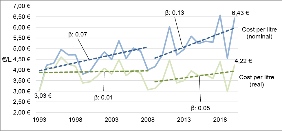
| Variable | Phase 1 (1993 - 2008) | Phase 2 (2009 - 2020) | ||||||
|---|---|---|---|---|---|---|---|---|
| Coefficients | Corrected R² | Coefficients | Corrected R² | |||||
| Coefficient | T-value | p-value | Coefficient | T-value | p-value | |||
| Cost per litre (€/L) | ||||||||
| nominal | 0.07 | 2.52 | <0.05 | 0.28 | 0.13 | 2.64 | <0.05 | 0.33 |
| real | 0.01 | 0.21 | 0.837 | -0.07 | 0.05 | 1.31 | 0.216 | 0.06 |
| Cost per ha (€/ha) | ||||||||
| nominal | 36.07 | 0.26 | 0.798 | -0.07 | 685.11 | 6.74 | <0.001 | 0.79 |
| real | -298.67 | -2.47 | <0.05 | 0.27 | 251.46 | 3.39 | <0.01 | 0.47 |
| Main Costs per ha (€/ha) | ||||||||
| Material costs | 44.78 | 1.02 | 0.326 | 0.00 | 164.18 | 4.16 | <0.01 | 0.58 |
| Labour costs | -12.67 | -0.65 | 0.530 | -0.04 | 302.99 | 10.87 | <0.001 | 0.91 |
| Financial costs | -16.70 | -1.71 | 0.111 | 0.12 | -36.14 | -13.24 | <0.001 | 0.94 |
| Labour Productivity (€/worker) | ||||||||
| nominal | 1,447.12 | 9.58 | <0.001 | 0.87 | 1,715.61 | 10.85 | <0.001 | 0.91 |
| real | 578.23 | 4.17 | <0.01 | 0.54 | 596.46 | 5.01 | <0.001 | 0.67 |
| Area Productivity (€/ha) | ||||||||
| nominal | 49.07 | 0.42 | 0.683 | -0.06 | 711.34 | 6.27 | <0.001 | 0.76 |
| real | -309.34 | -2.96 | <0.05 | 0.36 | 242.13 | 2.89 | <0.05 | 0.38 |
Cost per hectare
Costs per hectare shows a clear division into two phases: a stagnating or declining phase before the financial crisis, followed by an increasing cost phase thereafter. Visual inspection of Figure 10 suggests that costs per hectare continued to fall until around 2011, picking up only with the post-crisis recovery. For consistency, however, the 2008 cut-off is applied, which may underestimate the true slope of cost increases in the second phase.
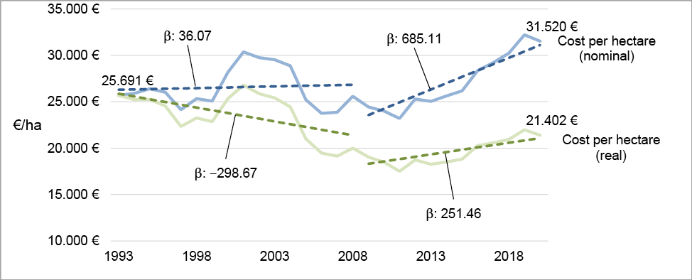
In the first phase nominal cost increased by €36 per hectare (not statistically significant), while real costs declined significantly by €299 per hectare and year (Table 2), driven primarily by reduced working hours per hectare (section 2.2.2). After 2008, nominal costs per hectare rose sharply, averaging €685 per hectare annually, with a more moderate real cost increase of €251 per hectare. Notably, real costs per hectare were 17% lower in 2020 than 28 years prior, indicating clear efficiency gains, while nominal costs per hectare increased by 23%, however. During the first phase, total cost development per ha did not vary significantly between the size groups. In the second phase, however, substantial differences were observed, as total costs for large wine estates increased at almost twice the average rate (Appendix C, Table 6).
Development of different cost types
For visual clarity, the analysis here focuses on nominal costs. Unsurprisingly, the two main cost drivers—material and labour costs per hectare—mirror the overall cost per hectare, stagnating in the first phase before the financial crisis and rising sharply thereafter (Figure 11, Table 2). During the first phase, material costs increased non-significantly by €45 per hectare per year, while in the second phase, they grew by an average of €164 per hectare. Labour costs initially declined by €13 per hectare annually, though not statistically significant, before rising sharply by €303 per hectare annually in the second phase. By 2020, labour costs per hectare were 82% higher than in 1993. Per-hectare labour costs increased most substantially for large wine estates, exceeding those of small and medium-sized businesses by 80%. Similarly, material costs for large estates rose at twice the average rate and were significantly higher than those of medium-sized wine estates, though not significantly different from those of small estates (Appendix C, Table 6).
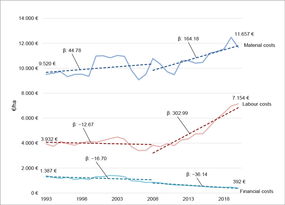
Financial costs, however, deviated from the overall cost trend, declining significantly by €36 per hectare during the second phase, as anticipated in section 2.3.1. Overall, financial costs fell by a factor of 3.5, from €1,387 to €392 per hectare. However, since financial costs constitute a very small portion of total costs, their decline could not offset the substantial increases in labour and material costs. There were no significant differences in the development of financial costs among the size groups.
4.2.2. Area Productivity and Labour Productivity
The Tier 2 KPIs of labour productivity and area productivity are influenced by the combined effects of Tier 1 KPIs. Labour productivity is affected by changes in yield, turnover per litre (price), and labour intensity, while area productivity is shaped by developments in yield and price. The structural breaks observed in the underlying KPIs are also evident in the graphs of labour and area productivity (Figure 12, Figure 13).
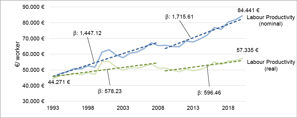
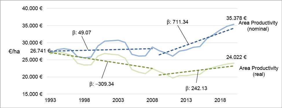
Labour productivity increased over the entire period (Figure 12). Since yield stabilised after 2008 (Figure 8) and turnover per litre grew more strongly (Figure 7), the annual increase in labour productivity was higher in the second phase (1,715 €/worker) compared to the first phase (1,447 €/worker). When adjusted for inflation, the trend is similar, yet with a reduced difference between the phases. Over the full 28-year period, nominal labour productivity nearly doubled, increasing by 91%, while the inflation-adjusted increase was more modest at 30%.
In the first phase, labour productivity developed similarly across all three size groups. However, in the second phase, large estates experienced a substantial improvement, increasing their labour productivity by 60% more than the average and 125% more than small estates (Appendix C, Table 6).
Due to declining yields (Figure 8), nominal area productivity remained stable in Phase 1 but decreased significantly in real terms, by €309 per hectare (Table 2). This decline in real land productivity is likely linked to the falling asset values of viticultural land during Phase 1 (Figure 4). When the decline in yield halted and real wine prices began to rise after 2008, area productivity increased significantly, both in nominal terms (€711 per hectare per year) and real terms (€242 per hectare per year). However, by the end of the observation period in 2020, real area productivity was 11% lower than in 1993. This decline is reflected in the significant negative slope of real area productivity, which fell by €194 per year over the entire period.
As with labour productivity, large estates achieved nearly twice the rate of area productivity growth compared to the average during the second phase, with a significantly greater increase than medium-sized wine estates. However, in the first phase, no significant differences between size groups were observed (Appendix C, Table 6).
The four highest-level KPIs in Tier 3 show similar development trends over time (Table 3). Both nominal and real values for all KPIs increased significantly during the first phase, peaking in 2008, the year of the financial crisis. They then declined until 2011, before rising again, albeit at a more moderate pace. The consistent increase during the first phase is reflected by a high level of explained variance, whereas the fluctuations in the second phase lead to a lower explained variance (Table 3). To avoid redundancy, only the operational result KPI is graphically presented here, as the other three KPIs follow essentially identical trends.
| Variable | Phase 1 (1993 - 2008) | Phase 2 (2009 - 2020) | ||||||
|---|---|---|---|---|---|---|---|---|
| Coefficients | Corrected R² | Coefficients | Corrected R² | |||||
| Coefficient | T-value | p-value | Coefficient | T-value | p-value | |||
| Profit per litre (€/L) | ||||||||
| nominal | 0.02 | 5.40 | <0.001 | 0.67 | 0.01 | 1.96 | 0.076 | 0.19 |
| real | 0.02 | 5.05 | <0.001 | 0.64 | 0.00 | 1.12 | 0.285 | 0.02 |
| Operational result per ha (€/ha) | ||||||||
| nominal | 159.84 | 4.76 | <0.001 | 0.61 | 59.21 | 1.42 | 0.182 | 0.08 |
| real | 133.12 | 4.44 | <0.001 | 0.57 | 21.48 | 0.69 | 0.505 | -0.05 |
| Return on Sales | 0.58 | 6.16 | <0.001 | 0.73 | 0.05 | 0.38 | 0.708 | -0.08 |
| Return on Equity | 0.38 | 5.60 | <0.001 | 0.68 | 0.11 | 1.43 | 0.180 | 0.08 |
The observed differences between size groups exhibit a consistent pattern across all Tier 3 key performance indicators (KPIs). In the first phase, the economic development of all three size groups was largely similar, with no statistically significant differences. However, in the second phase, only large wine estates demonstrated notable improvements in economic performance, significantly diverging from small and medium-sized businesses. The only exception was return on sales, where the substantial nominal difference was not statistically significant due to high variance (Appendix C, Table 6).
In 1993, wine estates made virtually no profit per litre, with a value of just €0.01. Nominal profit per litre then rose sharply, reaching €0.35 in 2008, before declining to €0.18 in 2011. By the end of the observation period, profit per litre had recovered to €0.42. The increase in profit per litre during the second phase was much smaller than in the first phase, where it grew by an average of €0.02 per litre per year. Over the entire second phase, the growth was not statistically different from zero (Table 3). During the second phase, only large estates experienced a significant annual increase in profit, rising by €0.03 per litre (Appendix C, Table 6).
4.3.2. Operational result per hectare
While the turnover per litre exclusively reflects the turnover generated by wine sales, the operational result per hectare also includes all secondary revenues generated by the wine estate. These include any form of gastronomic activity, events, subsidies, as well as revenues generated through rents and leases. As a result, wine estates, which are unable to cover costs per litre exclusively through wine sales can still generate a positive operational result per hectare through activity in said secondary branches of business.
The development of the operational result after imputed family wage is illustrated in Figure 14. The explanations for profit per litre discussed in section 4.3.1 apply here as well. The linear trend line for the first phase starts in the negative range, indicating that wine estates were unable to sufficiently remunerate their family workers during this period. Nominal operational results then increased sharply, peaking at €3,000 per hectare in 2008, before dropping to €1,100 in 2011 in the wake of the financial crisis. By the end of the observation period in 2020, the nominal operational result had recovered to approximately the 2008 level, at €3,051 per hectare. As a result, the slope for the second phase is not significant (Table 3). The real operational result follows a similar trend, with a slightly widening gap due to inflation.
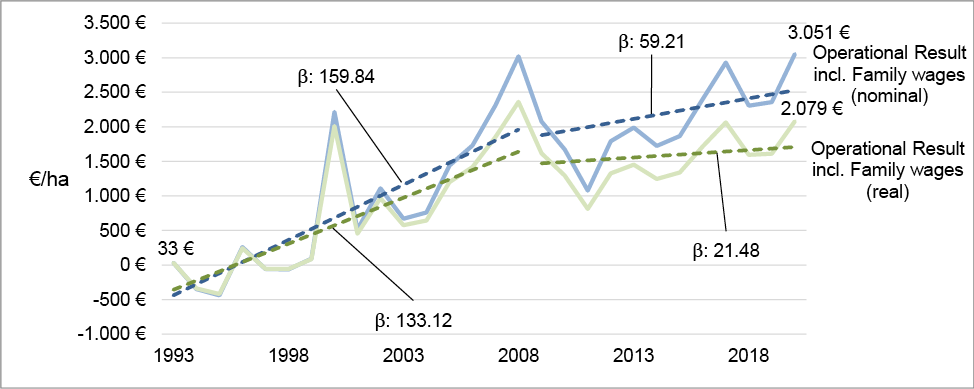
In the second phase, large wine estates were the only group to achieve a significant improvement in their operational result, with an average increase of €248 per hectare—nearly five times the overall average. This growth deviated significantly from that of small wine estates (Appendix C, Table 6).
4.3.3. Return on Sales and Equity
Return on sales and return on equity were both highly negative at the start of the observation period. In first phase, both increased significantly, with return on sales rising by 0.58% and return on equity by 0.38% annually (Table 3). Return on sales reached average positive values in 1998 and return on equity in 2002. Both peaked in 2008, the year of the financial crisis, at 8% and 5%, respectively, before declining sharply. By the end of the observation period, they had partially recovered to 7% for return on sales and 4.4% for return on equity. The developments during phase 2 were not statistically different from zero.
Analysing the development by size, large wine estates extended their positive trajectory from the first phase, achieving significant growth in return on sales and return on equity during the second phase, whereas small and medium-sized estates did not. Large estates increased their return on sales by 0.58% and their return on equity by 0.43%. While the increase in return on equity was significantly higher than in both other size groups, the increase in return on sales was not statistically significant due to substantial variation (Appendix C, Table 6).
This study descriptively analysed the long-term economic development of German wine estates over a 28-year period, based on 16 KPIs. The wine estates analysed represent approximately one-quarter of Germany’s wine production volume and span the entire value chain, from grape cultivation to the marketing of bottled wine. Similar to previous studies in agricultural economics [49,50,52], the analysis suggests a structural break in the economic development of wine estates following the 2008 financial crisis.
This section summarises the findings from the descriptive analysis, comparing the two phases—before and after the financial crisis—and relates them to the expectations from the literature. The discussion emphasises that each phase was driven by distinct economic factors.
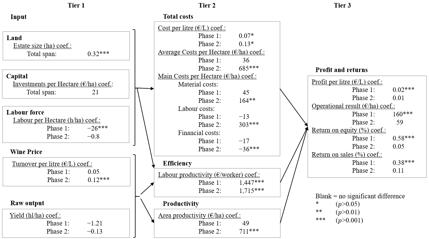
Figure 15 provides a summary of all coefficient results for the nominal KPI developments observed. Real values were disregarded for discussion to ensure comparability with previous literature, which solely takes nominal developments into consideration.
5.1. Economic development in phase 1 – prior the financial crisis
The primary positive driver in phase 1 was a 30% reduction in working hours per hectare (-26 h/ha annually), largely due to mechanisation and economies of scale (Figure 16). This aligns with trends in both German and international agriculture [6,17]. Constant investments per hectare can be attributed to the widespread use of rented machine harvesters, reducing the need for large capital outlays by wine estates. This contrasts with other agricultural sectors and challenges the expectation that larger businesses would drive up capital investments [6,29]. For wine estates, the benefits came from supply chain specialisation and using full harvesters provided by external service providers, who can leverage economies of scale more effectively than individual wine estates.
Additionally, as a minor positive driver, nominal turnover per litre increased by €0.05 annually, driven by value-added sales and marketing of bottled wine, while bulk wine prices lagged. Together, these factors resulted in a 48% increase in labour productivity. This is consistent with trends in the agricultural sector [15,36].
In addition to the two positive drivers, phase 1 was marked by negative factors, with declining yield being the most relevant. Unlike other agricultural sectors, wine estates did not benefit from yield improvements. Instead, yields consistently fell by 34% overall during the first phase (Figure 16). This decline reflects the shift of German wine estates from high-yield towards more in-demand grape varieties like Riesling [33]. The substantial yield drop, combined with only a minor increase in price, led to stagnating nominal and declining real area productivity (Table 1, Table 2). A marginal negative driver, was the rise in nominal costs, increasing by €36/ha and €0.07/litre annually (Figure 16).
Overall, the positive drivers—reduced labour input and modest increases in nominal prices—sufficiently offset these negative factors. During phase 1 (1993 to the 2008 financial crisis), wine estates significantly improved their profitability. Initially, wine estates were unable to properly compensate family workers, as indicated by a negative operational result after deducting family wages. However, this key performance indicator increased by €160/ha annually, and by the end of phase 1, wine estates had shifted from a deficit, with negative return on sales and equity, to a profitable position.
The economic drivers identified in the first phase applied regardless of wine estate size. The development of key performance indicators (KPIs) did not differ significantly among the three size groups, with the sole exception of the value of viticultural land as a fixed asset, which declined for small and medium-sized businesses but remained stable for large estates (Appendix C, Table 6).
5.2. Economic development in phase 2 – after the financial crisis
The increase in nominal prices per litre was the only significant positive driver in the post-financial crisis recovery period. Wine estates managed to raise prices by a total increase of 33%, primarily driven by value-added marketing, differentiation, and sales activities for bottled wine (Figure 17).
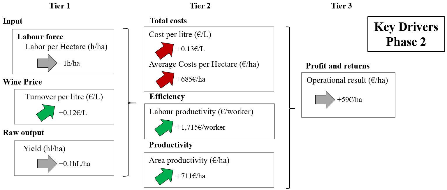
Labour hours, which had declined in the first phase, stagnated in phase 2 despite continued growth in business size (Figure 17). Any notable gains from mechanisation may have been offset by increased efforts in sales, marketing, and administration, as well as a growing focus on ecosystem services [58]. The rise in prices led to a 30% increase in labour productivity and raised area productivity by 31%, with yields remaining stable in phase 2.
The primary negative factor in phase 2 was the sharp rise in costs. Average costs per hectare grew by 32%, while costs per litre saw a similar increase of 31%. These increases were largely driven by rising minimum wages and higher material costs. Overall profitability, which had declined significantly after the financial crisis, recovered slowly, barely returning to 2008 levels by the end of phase 2, with price increases only just offsetting the rising costs (Figure 17).
In the second phase, wine estates of varying business sizes exhibited distinct performance patterns and growth trajectories. While the trends described above predominantly apply to small and medium-sized estates, the largest tertile continued to achieve profitability gains, as reflected in Tier 3 key performance indicators (Appendix C, Table 6). After 2009, however, large estates experienced more pronounced cost increases than their smaller counterparts, primarily due to rising labor and material expenses. This challenges the assumption that larger wine estates benefit from economies of scale, as suggested by Sellers & Alampi-Sottini [22]. Despite these cost pressures, large estates successfully offset rising expenses through substantial improvements in labour and land productivity. In particular, the marked increase in labor productivity suggests that larger estates leveraged workforce specialization to enhance operational efficiency.
Rather than benefiting from lower input costs, large wine estates appear to generate economic advantages by utilizing labor, land, and capital more productively, thereby creating greater value from their resources. These findings suggest that economic success in the wine sector under challenging conditions stems from specialization, which enables a more efficient and productive allocation of key input factors. The fact that large wine estates are significantly more successful has important implications for the future economic development and strategic adaptation of wine estates. Overall, the discrepancy between a positive development of the operational result, on average, even though the growth of average costs per litre exceeded that of the average turnover per litre, points to a reliance of wine estates on subsidies and revenues generated by secondary branches of business, such as gastronomy or events, as established in chapter 4.3.2. These implications for the future will be discussed in more detail in a separate discussion paper.
5.3. Limitations and Future Research
A limitation of this paper is sampling bias, as the data set is not fully representative of German wine estates. Future research could extend this approach to other countries. The study excludes other wine producers, such as grape growers, cooperatives, or large bottlers. Comparing the economic KPIs of wine estates with these other business types would provide valuable insights.
More successful wine estates are more likely to participate in the Geisenheim Business Analysis, while less successful ones may drop out or avoid participation. As a result, the data tends to reflect long-term survivors, as estates that close no longer submit data. This analysis does not account for panel effects.
Despite the overall robustness of the regression analysis, certain classical assumptions were not fully met. Specifically, the assumption of homoscedasticity was violated, as residual plots indicated non-constant variance. While extreme outliers were removed and diagnostic checks suggested limited influence on model results, it is still possible that heteroscedasticity affected the precision of the standard errors. Additionally, the residuals were not perfectly normally distributed, however, given that all sample sizes exceeded 100 observations, the Central Limit Theorem justifies the use of standard inferential procedures. These limitations should be considered when interpreting the confidence intervals and p-values, although the primary findings appear stable and reliable across model specifications.
The study focuses on descriptive analysis and linear trend estimation, without accounting for panel effects or sample heterogeneity over time. The structural shift following the global financial crisis has not been confirmed yet through statistical tests. Future research could include hazard/survival models or multivariate analysis for more detailed comparisons.
This study remains at an aggregate level, analysing KPIs across all participating wine estates without examining specific strategies employed by individual businesses. Future research could explore the strategies of the most successful estates to understand which decisions and actions have driven their success. The paper is also limited in scope by only interpreting past data, due to a lack of availability of more recent data, which could be included for further analysis in the future.
A separate discussion paper will apply these findings to the economic developments after 2020 and derive recommendations for the future strategic management of wine estates in Germany.
This study focussed on the long-term economic developments of German wine estates before and after the 2008 financial crisis. From 1993-2008, estates benefited from mechanisation, reducing labour per hectare and offsetting declining yields, thus improving productivity and profitability, especially for larger wine estates. From 2009 to 2020, escalating labour and material costs negated price increases, culminating in stagnating profitability. However, the increase of economic performance of large wine estates versus the stagnation and decline within small to medium estates in the latter period, suggests a positive effect related to economies of scale through size increase. Moving forward, the challenges of rising costs, inflation and a declining global wine consumption, leave wine estates in progressively dire straits. To adapt, German wine estates must further embrace mechanisation and the investment into labour-saving technologies to counterbalance increasing costs, while also reconsidering yield management strategies and optimizing their positioning within the market. All in all, this study provides lessons from past developments as a future roadmap for wine estates to enhance their efficiency and productivity, remain persistent in the face of current economic challenges, and ensure long-term economic sustainability in the future.
[1] R. del Rey, S. Loose, State of the International Wine Market in 2022: New market trends for wines require new strategies, WEP 12 (2023) 3–18. https://doi.org/10.36253/wep-14758.
[2] OIV, The State of the World Vine and Wine Sector in 2023 report, 2024. https://t.ly/baZXj (accessed 30 May 2024).
[3] B. Richter, J. Hanf, KEEPING UP WITH COMPETITORS, 1st Conference of the European Assosiation of Wine Economists (2022) 35–37.
[4] S.M. Loose, E. Pabst, Current state of the German and international wine markets, German Journal of Agricultural Economics - GJAE, 2018.
[5] DWI, 22’/23 Deutscher Wein Statistik, 2022. https://t.ly/XGXKY (accessed 8 February 2023).
[6] J.M. MacDonald, Tracking the Consolidation of U.S. Agriculture, Applied Eco Perspectives Pol 42 (2020) 361–379. https://doi.org/10.1002/aepp.13056.
[7] S. Zeng, F. Zhu, F. Chen, M. Yu, S. Zhang, Y. Yang, Assessing the Impacts of Land Consolidation on Agricultural Technical Efficiency of Producers: A Survey from Jiangsu Province, China, Sustainability 10 (2018) 2490. https://doi.org/10.3390/su10072490.
[8] R. del Rey, S. Loose, State of the International Wine Markets in 2023: The wine market at a crossroads: Temporary or structural challenges?, WEP (2024).
[9] M. Boehlje, J. Akridge, D. Downey, Restructuring agribusiness for the 21st century, Agribusiness 11 (1995) 493–500. https://doi.org/10.1002/1520-6297(199511/12)11:6<493:AID-AGR2720110602>3.0.CO;2-G.
[10] DWI, Mafo-Newsletter 01/2024, 2024. https://t.ly/Lo37D (accessed 22 May 2024).
[11] DWI, ‘23/ ‘24 Deutscher Wein Statistik, 2023. https://t.ly/QTxnj (accessed 5 December 2023).
[12] M. Berner, DWI-Sonderbericht Weinkonsumbilanz 2021/22, Deutscher Weinbauverband e.V., 2023.
[13] M. Tafel, G. Szolnoki, Estimating the economic impact of tourism in German wine regions, Int J Tourism Res 22 (2020) 788–799. https://doi.org/10.1002/jtr.2380.
[14] A.W. Bennett, S.M. Loose, Benchmarking Economic Sustainability: What Factors Explain Heterogeneity between Wine Businesses?, Sustainability 15 (2023) 16686. https://doi.org/10.3390/su152416686.
[15] K. Ryszard, Agricultural Productivity in Poland in the Context of Structural Changes in the Sector in 2002-2016, Economic Sciences for Agribusiness and Rural Economy (2018) 109–115. https://doi.org/10.22630/ESARE.2018.2.13.
[16] S. Huettel, A. Margarian, Structural change in the West German agricultural sector, Agricultural Economics 40 (2009) 759–772. https://doi.org/10.1111/j.1574-0862.2009.00413.x.
[17] BMEL, Landwirtschaftliche Betriebe, 2024. https://t.ly/C6KY0 (accessed 4 January 2024).
[18] A. Silberston, Economies of Scale in Theory and Practice, The Economic Journal 82 (1972) 369. https://doi.org/10.2307/2229943.
[19] G.J. Stigler, The Economies of Scale, The Journal of Law and Economics 1 (1958) 54–71. https://doi.org/10.1086/466541.
[20] R. Sellers-Rubio, V. Alampi Sottini, S. Menghini, Productivity growth in the winery sector: evidence from Italy and Spain, Intl Jnl of Wine Business Res 28 (2016) 59–75. https://doi.org/10.1108/IJWBR-05-2015-0019.
[21] S. Tudisca, A.M. Di Trapani, F. Sgroi, R. Testa, The Cost Advantage of Sicilian Wine Farms, American Journal of Applied Sciences 10 (2013) 1529–1536. https://doi.org/10.3844/ajassp.2013.1529.1536.
[22] R. Sellers, V. Alampi-Sottini, The influence of size on winery performance: Evidence from Italy, Wine Economics and Policy 5 (2016) 33–41. https://doi.org/10.1016/j.wep.2016.03.001.
[23] A. Corsi, S. Mazzarino, E. Pomarici, The Italian Wine Industry, in: A. Alonso Ugaglia (Ed.), The Palgrave Handbook of Wine Industry Economics, Palgrave Macmillan US, Cham, 2019, pp. 47–76.
[24] L.M. Albisu, C. Escobar, R. del Rey, J.M. Gil Roig, The Spanish Wine Industry, in: A. Alonso Ugaglia (Ed.), The Palgrave Handbook of Wine Industry Economics, Palgrave Macmillan US, Cham, 2019, pp. 77–103.
[25] E. Pomarici, A. Corsi, S. Mazzarino, R. Sardone, The Italian Wine Sector: Evolution, Structure, Competitiveness and Future Challenges of an Enduring Leader, Ital Econ J 7 (2021) 259–295. https://doi.org/10.1007/s40797-021-00144-5.
[26] M. Boehlje, Alternative models of structural change in agriculture and related industries, Agribusiness 8 (1992) 219–231. https://doi.org/10.1002/1520-6297(199205)8:3<219:AID-AGR2720080303>3.0.CO;2-T.
[27] B. Perretti, Economic sustainability of quality wine districts in the South of Italy. The case of Vulture, IJGSB 11 (2020) 356. https://doi.org/10.1504/IJGSB.2020.110793.
[28] BMEL, Tabellen zur Landwirtschaft, 2024. https://t.ly/p9qoL (accessed 4 January 2024).
[29] T. Filipiak, L. Wicki, Is the Structure of Polish Agriculture Changing? A Comparison Based on the Results of Recent General Agricultural Census, Annals PAAAE XXIV (2022) 37–53. https://doi.org/10.5604/01.3001.0015.7103.
[30] J.-P. Chavas, On the economics of agricultural production*, Australian Journal of Agricultural and Resource Economics 52 (2008) 365–380. https://doi.org/10.1111/j.1467-8489.2008.00442.x.
[31] D. Kirschke, A. Häger, J.C. Schmid, New Trends and Drivers for Agricultural Land Use in Germany, in: Sustainable Land Management in a European Context, Springer, Cham, 2021, pp. 39–61.
[32] S.L. Wang, P. Heisey, D. Schimmelpfennig, V.E. Ball, Agricultural Productivity Growth in the United States: Measurement, Trends, and Drivers, 2015.
[33] Federal Statistical Office of Germany, Rebflächen nach den wichtigsten Rebsorten im Zeitvergleich, 2023. https://t.ly/JONBx (accessed 22 January 2024).
[34] BMEL-Statistik, Erntemenge an Weinmost, Weinmostertrag je Hektar, Rebfläche im Ertrag: Deutschland, Jahre, Art des Weinmosts, 2024. https://t.ly/FAQgD (accessed 26 March 2024).
[35] Statista, Landwirtschaftliche Betriebsmittel - Index der Einkaufspreise bis 2023 | Statista, 2024. https://t.ly/IbIa1 (accessed 15 February 2024).
[36] BMEL-Statistik, Buchführungsergebnisse Landwirtschaft 2006/07, 2024. https://t.ly/GZ9xf (accessed 15 February 2024).
[37] BMEL-Statistik, Buchführungsergebnisse Landwirtschaft 2021/22, 2024. https://t.ly/netHb (accessed 15 February 2024).
[38] German Federal Bank, Lange Zeitreihen zur Wirtschaftsentwicklung in Deutschland: Geld und Kapitalmarkt, 2024. https://t.ly/Y9fxw (accessed 17 September 2024).
[39] P. Groenewegen, Division of Labour, in: The New Palgrave Dictionary of Economics, Palgrave Macmillan, London, 2019, pp. 1–11.
[40] X. Yang, Economic Development and the Division of Labor, John Wiley & Sons Incorporated, Newark, 2003.
[41] S. Kim, Labor Specialization and the Extent of the Market, Journal of Political Economy 97 (1989) 692–705. https://doi.org/10.1086/261622.
[42] J. Bereżnicka, Sources of Return on Equity in Economically Diversified Agriculture of the European Union Countries, Zagadnienia Ekonomiki Rolnej 356 (2018) 76–93. https://doi.org/10.30858/zer/94477.
[43] BMEL-Statistik, Archiv Buchführungsergebnisse Landwirtschaft, 2024. https://t.ly/Pr0cL (accessed 15 February 2024).
[44] Z. Guo, Y. Feng, T. Gries, Changes of China’s agri-food exports to Germany caused by its accession to WTO and the 2008 financial crisis, China Agricultural Economic Review 7 (2015) 262–279. https://doi.org/10.1108/CAER-11-2013-0152.
[45] R. Crescenzi, D. Luca, S. Milio, The geography of the economic crisis in Europe: national macroeconomic conditions, regional structural factors and short-term economic performance, Cambridge J Regions Econ Soc 9 (2016) 13–32. https://doi.org/10.1093/cjres/rsv031.
[46] L. Ball, Long-term damage from the Great Recession in OECD countries, European Journal of Economics and Economic Policies: Intervention 11 (2014) 149–160. https://doi.org/10.4337/ejeep.2014.02.02.
[47] L. Dijkstra, E. Garcilazo, P. McCann, The effects of the global financial crisis on European regions and cities, Journal of Economic Geography 15 (2015) 935–949. https://doi.org/10.1093/jeg/lbv032.
[48] E. Hernández, H. Kriesi, The electoral consequences of the financial and economic crisis in Europe, European Journal of Political Research 55 (2015) 203–224. https://doi.org/10.1111/1475-6765.12122.
[49] L. Sdrolias, A. Semos, K. Mattas, E. Tsakiridou, A. Michailides, M. Partalidou, D. Tsiotas, Assessing the Agricultural Sector’s Resilience to the 2008 Economic Crisis: The Case of Greece, Agriculture 12 (2022) 174. https://doi.org/10.3390/agriculture12020174.
[50] G.A. Oladosu, K.L. Kline, J.W.A. Langeveld, Structural Break and Causal Analyses of U.S. Corn Use for Ethanol and Other Corn Market Variables, Agriculture 11 (2021) 267. https://doi.org/10.3390/agriculture11030267.
[51] Y. Tsuchiya, Linkages among commodity futures prices in the recent financial crisis: An application of cointegration tests with a structural break, Cogent Economics & Finance 3 (2015) 1012436. https://doi.org/10.1080/23322039.2015.1012436.
[52] A. Kalsie, A. Arora, Structural break, US financial crisis and macroeconomic time series: evidence from BRICS economies, Transnational Corporations Review 11 (2019) 250–264. https://doi.org/10.1080/19186444.2018.1475087.
[53] A.W. Bennett, S. Müller Loose, User-Centered Development of an Online Dashboard Tool for Economic Sustainability for Small and Medium Enterprises, Sustainability 16 (2024) 557. https://doi.org/10.3390/su16020557.
[54] M. Ghosh, Structural Breaks and Performance in Agriculture, in: M. Ghosh (Ed.), Liberalization, Growth and Regional Disparities in India, Springer, India, 2013, pp. 83–107.
[55] G. Casella, R.L. Berger, Statistical inference, Second edition, CENGAGE Learning, Andover, Melbourne, Mexico City, Stamford, CT, Toronto, Hong Kong, New Delhi, Seoul, Singapore, Tokyo, 2002.
[56] A.W. van der Vaart, Asymptotic statistics, First paperback edition, eighth. printing, Cambridge University Press, Cambridge, New York, 2007.
[57] J. Fox, Applied regression analysis and generalized linear models, Third edition, Sage, Los Angeles, London, New Delhi, Singapore, Washington DC, Boston, 2016.
[58] Federal Statistical Office of Germany, Deutlicher Zuwachs an Ökobetrieben und ökologisch bewirtschafteten Flächen im letzten Jahrzehnt, 2023. https://t.ly/s9TWA (accessed 18 September 2024).
| Year | Sample size | Small (ha) | Medium (ha) | Large (ha) | |||
|---|---|---|---|---|---|---|---|
| Minimum | Maximum | Minimum | Maximum | Minimum | Maximum | ||
| 1993 | 106 | 1.2 | 5.2 | 5.2 | 8.4 | 8.4 | 22.4 |
| 1994 | 107 | 1.7 | 5.9 | 6.0 | 9.4 | 9.5 | 32.0 |
| 1995 | 114 | 1.5 | 6.0 | 6.1 | 8.9 | 9.0 | 24.7 |
| 1996 | 129 | 2.2 | 6.5 | 6.6 | 10.2 | 10.2 | 24.7 |
| 1997 | 153 | 1.7 | 6.9 | 6.9 | 10.8 | 10.9 | 28.5 |
| 1998 | 172 | 1.8 | 7.2 | 7.3 | 11.5 | 11.5 | 40.4 |
| 1999 | 181 | 1.8 | 7.4 | 7.4 | 11.7 | 11.7 | 35.4 |
| 2000 | 110 | 2.2 | 7.6 | 7.6 | 10.8 | 11.0 | 26.7 |
| 2001 | 117 | 2.1 | 7.2 | 7.2 | 11.2 | 11.2 | 29.0 |
| 2002 | 131 | 2.3 | 7.0 | 7.1 | 11.2 | 11.2 | 36.6 |
| 2003 | 125 | 1.5 | 7.1 | 7.2 | 10.8 | 10.9 | 36.2 |
| 2004 | 140 | 1.9 | 7.2 | 7.2 | 11.7 | 11.7 | 36.3 |
| 2005 | 159 | 2.7 | 9.7 | 9.7 | 13.6 | 13.7 | 67.8 |
| 2006 | 185 | 3.1 | 10.0 | 10.2 | 14.4 | 14.4 | 47.0 |
| 2007 | 223 | 2.1 | 9.7 | 9.7 | 14.4 | 14.5 | 70.0 |
| 2008 | 282 | 0.6 | 8.6 | 8.6 | 14.2 | 14.4 | 49.8 |
| 2009 | 292 | 2.0 | 8.6 | 8.7 | 14.5 | 14.5 | 55.7 |
| 2010 | 311 | 2.1 | 8.8 | 8.8 | 15.1 | 15.1 | 50.5 |
| 2011 | 319 | 1.5 | 8.8 | 8.8 | 15.2 | 15.3 | 57.4 |
| 2012 | 300 | 2.3 | 9.8 | 9.8 | 15.7 | 15.7 | 57.8 |
| 2013 | 304 | 2.3 | 9.4 | 9.4 | 15.5 | 15.6 | 50.9 |
| 2014 | 309 | 2.1 | 9.8 | 9.8 | 16.3 | 16.4 | 62.8 |
| 2015 | 304 | 0.5 | 9.7 | 9.7 | 16.9 | 17.0 | 60.3 |
| 2016 | 300 | 0.5 | 10.4 | 10.4 | 17.0 | 17.2 | 72.6 |
| 2017 | 309 | 0.5 | 10.0 | 10.2 | 17.0 | 17.1 | 67.0 |
| 2018 | 310 | 0.5 | 10.1 | 10.1 | 16.3 | 16.6 | 58.6 |
| 2019 | 304 | 2.3 | 9.9 | 9.9 | 16.6 | 16.7 | 69.0 |
| 2020 | 279 | 2.3 | 10.2 | 10.2 | 17.9 | 18.0 | 72.6 |
| Total timespan (1993 - 2020) | |||||
|---|---|---|---|---|---|
| Coefficients | hs | Conf. Int. 95% | |||
| Variable | Coefficient | p-value | lower | upper | |
| Business Size (ha) | 0.32 | <0.001 | - | - | |
| Small | 0.09 | <0.001 | c | 0.07 | 0.12 |
| Medium | 0.25 | <0.001 | b | 0.22 | 0.28 |
| Large | 0.62 | <0.001 | a | 0.56 | 0.68 |
| % Full-time employees | 0.85 | <0.001 | |||
| Small | 0.75 | <0.001 | b | 0.68 | 0.82 |
| Medium | 0.77 | <0.001 | b | 0.67 | 0.87 |
| Large | 1.00 | <0.001 | a | 0.90 | 1.10 |
| Variable | Phase 1 (1993 - 2008) | Phase 2 (2009 - 2020) | ||||||||
|---|---|---|---|---|---|---|---|---|---|---|
| Coefficients | hs | Conf. Int. 95% | Coefficients | hs | Conf. Int. 95% | |||||
| Coefficient | p-value | lower | upper | Coefficient | p-value | lower | upper | |||
| Viticultural area | -343 | <0.05 | - | - | -56 | 0.467 | - | - | ||
| Small | -635 | <0.001 | b | -934 | -336 | -323 | <0.05 | bc | -557 | -90 |
| Medium | -600 | <0.05 | b | -1103 | -98 | 291 | <0.05 | a | 10 | 572 |
| Large | 199 | 0.260 | a | -164 | 562 | -201 | 0.313 | ab | -624 | 221 |
| Cost per ha (€/ha) | ||||||||||
| nominal | 0.11 | 0.999 | 671 | <0.001 | ||||||
| Small | 76.01 | 0.551 | -191 | 343 | 739 | <0.001 | b | 618 | 859 | |
| Medium | 24.24 | 0.865 | -275 | 324 | 470 | <0.001 | b | 284 | 656 | |
| Large | -98.33 | -0.668 | -414 | 217 | 1152 | <0.001 | a | 874 | 1430 | |
| Main Costs per ha (€/ha) | ||||||||||
| Material costs | 57 | 0.173 | 155 | <0.01 | ||||||
| Small | 95 | <0.05 | 10 | 180 | 180 | <0.001 | ab | 102 | 258 | |
| Medium | 108 | <0.05 | 8 | 208 | 101 | <0.05 | b | 13 | 188 | |
| Large | -36 | 0.505 | -148 | 76 | 309 | <0.001 | a | 220 | 398 | |
| Labour costs | -12 | 0.465 | 296 | <0.001 | ||||||
| Small | 11 | 0.581 | -30 | 52 | 256 | <0.001 | b | 225 | 287 | |
| Medium | -22 | 0.163 | -55 | 10 | 256 | <0.001 | b | 188 | 325 | |
| Large | -23 | 0.475 | -91 | 44 | 459 | <0.001 | a | 375 | 543 | |
| Labour Productivity (€/worker) | ||||||||||
| nominal | 1457 | <0.001 | 1713 | <0.001 | ||||||
| Small | 1304 | <0.001 | 940 | 1668 | 1239 | <0.001 | b | 998 | 1480 | |
| Medium | 1705 | <0.001 | 1368 | 2042 | 1634 | <0.001 | b | 1286 | 1982 | |
| Large | 1359 | <0.001 | 831 | 1886 | 2783 | <0.001 | a | 2271 | 3295 | |
| Area Productivity (€/ha) | ||||||||||
| nominal | 37 | 0.726 | 697 | <0.001 | ||||||
| Small | 139 | 0.215 | -91 | 369 | 806 | <0.001 | ab | 593 | 1019 | |
| Medium | 58 | 0.636 | -200 | 317 | 503 | <0.001 | b | 308 | 699 | |
| Large | -83 | 0.550 | -373 | 208 | 1179 | <0.001 | a | 902 | 1455 | |
| Profit per litre (€/L) | ||||||||||
| nominal | 0.02 | <0.001 | 0.01 | 0.103 | ||||||
| Small | 0.04 | <0.001 | 0.02 | 0.05 | 0.00 | 0.928 | b | -0.014 | 0.015 | |
| Medium | 0.02 | <0.001 | 0.01 | 0.03 | 0.01 | 0.263 | ab | -0.007 | 0.022 | |
| Large | 0.02 | <0.01 | 0.01 | 0.03 | 0.03 | <0.01 | a | 0.017 | 0.052 | |
| Operational result per ha (€/ha) | ||||||||||
| nominal | 186 | <0.001 | 53 | 0.237 | ||||||
| Small | 306 | <0.001 | 179 | 432 | 25 | 0.571 | b | -69 | 118 | |
| Medium | 148 | <0.001 | 75 | 221 | 63 | 0.197 | ab | -39 | 164 | |
| Large | 110 | <0.01 | 34 | 185 | 248 | <0.001 | a | 152 | 344 | |
| Return on Equity | 0.44 | <0.001 | 0.10 | 0.242 | ||||||
| Small | 0.66 | <0.001 | 0.45 | 0.87 | 0.11 | 0.249 | b | -0.09 | 0.31 | |
| Medium | 0.40 | <0.001 | 0.25 | 0.54 | 0.04 | 0.705 | b | -0.20 | 0.28 | |
| Large | 0.33 | <0.01 | 0.16 | 0.51 | 0.43 | <0.001 | a | 0.32 | 0.55 | |